Geographic distance
The first post of this year 2020, I will dedicate to a question that I was recently asked. The question was how to calculate the shortest distance between different points and how to know which is the closest point. When we work with spatial data in R, currently the easiest thing is to use the sf package in combination with the tidyverse collection of packages. We also use the units package which is very useful for working with units of measurement.
Packages
| Package | Description |
|---|---|
| tidyverse | Collection of packages (visualization, manipulation): ggplot2, dplyr, purrr, etc. |
| sf | Simple Feature: import, export and manipulate vector data |
| units | Support for measurement units in R vectors, matrices and arrays: propagation, conversion, derivation |
| maps | Draw geographical maps |
| rnaturalearth | Hold and facilitate interaction with Natural Earth map data |
# install the necessary packages
if(!require("tidyverse")) install.packages("tidyverse")
if(!require("units")) install.packages("units")
if(!require("sf")) install.packages("sf")
if(!require("maps")) install.packages("maps")
if(!require("rnaturalearth")) install.packages("rnaturalearth")

# load packages
library(maps)
library(sf)
library(tidyverse)
library(units)
library(rnaturalearth)
Measurement units
The use of vectors and matrices with the units class allows us to calculate and transform units of measurement.
# length
l <- set_units(1:10, m)
l
## Units: [m]
## [1] 1 2 3 4 5 6 7 8 9 10# convert units
set_units(l, cm)## Units: [cm]
## [1] 100 200 300 400 500 600 700 800 900 1000# sum different units
set_units(l, cm) + l## Units: [cm]
## [1] 200 400 600 800 1000 1200 1400 1600 1800 2000# area
a <- set_units(355, ha)
set_units(a, km2)## 3.55 [km2]# velocity
vel <- set_units(seq(20, 50, 10), km/h)
set_units(vel, m/s)## Units: [m/s]
## [1] 5.555556 8.333333 11.111111 13.888889Capital cities of the world
We will use the capital cities of the whole world with the objective of calculating the distance to the nearest capital city and indicating the name/country.
# set of world cities with coordinates
head(world.cities) # from the maps package
## name country.etc pop lat long capital
## 1 'Abasan al-Jadidah Palestine 5629 31.31 34.34 0
## 2 'Abasan al-Kabirah Palestine 18999 31.32 34.35 0
## 3 'Abdul Hakim Pakistan 47788 30.55 72.11 0
## 4 'Abdullah-as-Salam Kuwait 21817 29.36 47.98 0
## 5 'Abud Palestine 2456 32.03 35.07 0
## 6 'Abwein Palestine 3434 32.03 35.20 0To convert points with longitude and latitude into a spatial object of class sf, we use the function st_as_sf(), indicating the coordinate columns and the coordinate reference system (WSG84, epsg: 4326).
# convert the points into an sf object with CRS WSG84
cities <- st_as_sf(world.cities, coords = c("long", "lat"), crs = 4326)
cities
## Simple feature collection with 43645 features and 4 fields
## Geometry type: POINT
## Dimension: XY
## Bounding box: xmin: -178.8 ymin: -54.79 xmax: 179.81 ymax: 78.93
## Geodetic CRS: WGS 84
## First 10 features:
## name country.etc pop capital geometry
## 1 'Abasan al-Jadidah Palestine 5629 0 POINT (34.34 31.31)
## 2 'Abasan al-Kabirah Palestine 18999 0 POINT (34.35 31.32)
## 3 'Abdul Hakim Pakistan 47788 0 POINT (72.11 30.55)
## 4 'Abdullah-as-Salam Kuwait 21817 0 POINT (47.98 29.36)
## 5 'Abud Palestine 2456 0 POINT (35.07 32.03)
## 6 'Abwein Palestine 3434 0 POINT (35.2 32.03)
## 7 'Adadlay Somalia 9198 0 POINT (44.65 9.77)
## 8 'Adale Somalia 5492 0 POINT (46.3 2.75)
## 9 'Afak Iraq 22706 0 POINT (45.26 32.07)
## 10 'Afif Saudi Arabia 41731 0 POINT (42.93 23.92)In the next step, we filter by the capital cities encoded in the column capital with 1. The advantage of the sf package is the possibility of applying functions of the tidyverse collection to manipulate the attributes. In addition, we add a column with new labels using the str_c() function of the stringr package, which is similar to that of R Base paste().
# filter the capital cities
capitals <- filter(cities, capital == 1)

# create a new label combining name and country
capitals <- mutate(capitals, city_country = str_c(name, " (", country.etc, ")"))

capitals
## Simple feature collection with 230 features and 5 fields
## Geometry type: POINT
## Dimension: XY
## Bounding box: xmin: -176.13 ymin: -51.7 xmax: 179.2 ymax: 78.21
## Geodetic CRS: WGS 84
## First 10 features:
## name country.etc pop capital geometry
## 1 'Amman Jordan 1303197 1 POINT (35.93 31.95)
## 2 Abu Dhabi United Arab Emirates 619316 1 POINT (54.37 24.48)
## 3 Abuja Nigeria 178462 1 POINT (7.17 9.18)
## 4 Accra Ghana 2029143 1 POINT (-0.2 5.56)
## 5 Adamstown Pitcairn 51 1 POINT (-130.1 -25.05)
## 6 Addis Abeba Ethiopia 2823167 1 POINT (38.74 9.03)
## 7 Agana Guam 1041 1 POINT (144.75 13.47)
## 8 Algiers Algeria 2029936 1 POINT (3.04 36.77)
## 9 Alofi Niue 627 1 POINT (-169.92 -19.05)
## 10 Amsterdam Netherlands 744159 1 POINT (4.89 52.37)
## city_country
## 1 'Amman (Jordan)
## 2 Abu Dhabi (United Arab Emirates)
## 3 Abuja (Nigeria)
## 4 Accra (Ghana)
## 5 Adamstown (Pitcairn)
## 6 Addis Abeba (Ethiopia)
## 7 Agana (Guam)
## 8 Algiers (Algeria)
## 9 Alofi (Niue)
## 10 Amsterdam (Netherlands)Calculate distances
Geographical distance (Euclidean or greater circle) is calculated with the st_distance() function, either between two points, between one point and others or between all points. In the latter case we obtain a symmetric matrix of distances (NxN), taken pairwise between the elements of the capital city set. In the diagonal we find the combinations between the same points giving all null values.
| A | B | C | |
| A | 0 | 255 | 345 |
| B | 255 | 0 | 142 |
| C | 345 | 142 | 0 |
For instance, when we want to know the distance from Amsterdam to Abu Dhabi, Washington and Tokyo we pass two spatial objects.
# calculate distance
dist_amsterdam <- st_distance(slice(capitals, 10),
                              slice(capitals, c(2, 220, 205)))

dist_amsterdam # distance in meters
## Units: [m]
## [,1] [,2] [,3]
## [1,] 5163124 6187634 9293710The result is a matrix with a single row or column (depending on the order of the spatial objects) with a class of units. Thus it is possible to convert easily to another unit of measure. If we want to obtain a vector without class units, we only have to apply the function as.vector().
# change from m to km
set_units(dist_amsterdam, "km")
## Units: [km]
## [,1] [,2] [,3]
## [1,] 5163.124 6187.634 9293.71# units class to vector
as.vector(dist_amsterdam)## [1] 5163124 6187634 9293710In the second step, we estimate the distance matrix between all the capital cities. It is important to convert the null values to NA to subsequently obtain the correct matrix index.
# calculate distance
m_distance <- st_distance(capitals)

# matrix
dim(m_distance)
## [1] 230 230# change m to km
m_distance_km <- set_units(m_distance, km)
# replace the distance of 0 m with NA
m_distance_km[m_distance_km == set_units(0, km)] <- NAunits class, it is necessary to use the same class to be able to make logical queries. For example, set_units(1, m) == set_units(1, m) vs. set_units(1, m) == 1.
To obtain the shortest distance, in addition to its position, we use the apply () function which in turn allows us to apply the function which.min() and min() on each row. It would also be possible to use the function on columns giving the same result. Finally, we add the results as new columns with the mutate() function. The indices in pos allow us to obtain the names of the nearest cities.
# get the index (position) of the city and the distance
pos <- apply(m_distance_km, 1, which.min)
dist <- apply(m_distance_km, 1, min, na.rm = TRUE)
# add the distance and get the name of the city
capitals <- mutate(capitals, nearest_city = city_country[pos],
geometry_nearest = geometry[pos],
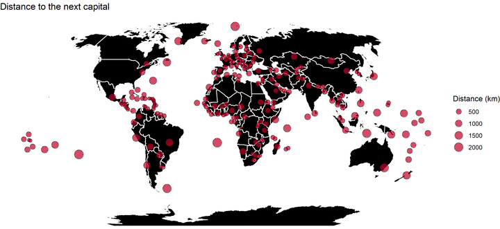
distance_city = dist)Map of distances to the next capital city
Finally, we build a map representing the distance in proportional circles. To do this, we use the usual grammar of ggplot() by adding the geometry geom_sf(), first for the world map as background and then for the cities. In aes() we indicate, with the argument size = distance_city, the variable which we want to map proportionally. The theme_void() function removes all style elements. In addition, we define with the function coord_sf() a new projection indicating the proj4 format.
# world map
world <- ne_countries(scale = 10, returnclass = "sf")

# map
ggplot(world) +
   geom_sf(fill = "black", colour = "white") +
   geom_sf(data = capitals,
           aes(size = distance_city),
           alpha = 0.7,
           fill = "#bd0026",
           shape = 21,
           show.legend = 'point') +
   coord_sf(crs = "+proj=robin +lon_0=0 +x_0=0 +y_0=0 +ellps=WGS84 +datum=WGS84 +units=m +no_defs") +
  labs(size = "Distance (km)", title = "Distance to the next capital city") +
  theme_void()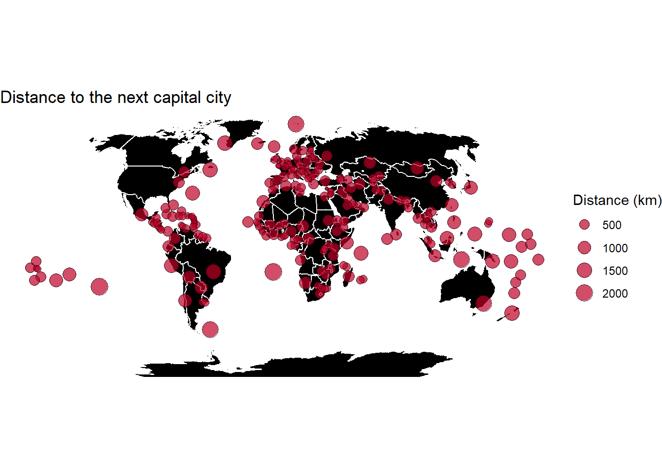
![]()