# install the packages if necessary

if (!require("tidyverse")) install.packages("tidyverse")
if (!require("mapSpain")) install.packages("mapSpain")
if (!require("sf")) install.packages("sf")
if (!require("janitor")) install.packages("janitor")
if (!require("patchwork")) install.packages("patchwork")

# packages

library(tidyverse)
library(readxl)
library(sf)
library(mapSpain)
library(janitor)
library(patchwork)Always normalize your data
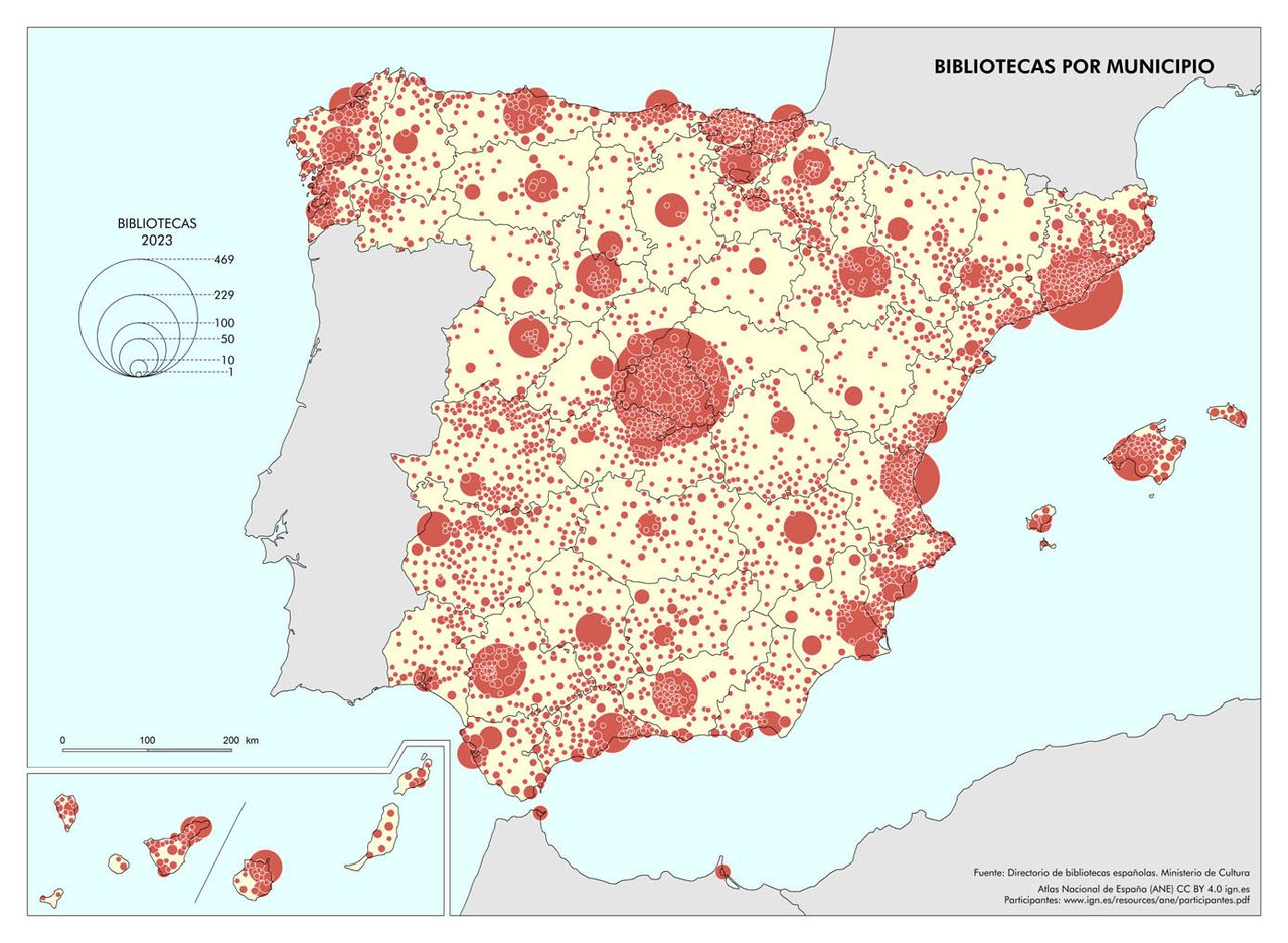
I recently came across a map from the National Atlas of Spain showing the number of libraries by municipality. However, one thing directly caught my attention. There’s a saying that many maps show only the population, and this seems to be the case here. The map does not provide any remarkable information about the distribution of libraries; it merely shows where the most people live. It’s a very common pitfall. There are many phenomena that depend on population. It can be assumed that the number of libraries largely depends on the number of inhabitants in each municipality. Therefore, we see cities like Madrid, Barcelona, Seville, Valencia, and many provincial capitals with a higher number of libraries.
A good practice is always to normalize variables that depend highly on the population. Pairing absolute numbers with normalized data is also beneficial. However, there are cases where the absolute number may be of interest. For instance, when considering poverty, normalized numbers may obscure the significant number of individuals affected.
Normalization of population-dependent variables can be performed in different ways, depending on the context and type of data. In our case, it involves dividing the number of libraries by the total population. To avoid very small numbers, it is common to multiply by a fixed population, such as 10,000. Another alternative, but not in this case, would be the use of percent.
\[ \text{Libraries per 10,000 inhabitants} = \left( \frac{\text{Number of libraries}}{\text{Total population}}\right) \times 10,000 \]
If you divide the other way around, it gives you a different perspective. You are calculating how many people, on average, have access to a single library.
\[ \text{Inhabitants per library} = \frac{\text{Total population}}{\text{Number of libraries}} \]
Lets get to work!
Packages
| Package | Description |
|---|---|
| tidyverse | Collection of packages (visualization, manipulation): ggplot2, dplyr, purrr, etc. |
| mapSpain | Administrative boundaries of Spain at different levels |
| sf | Simple Feature: import, export and manipulate vector data |
| janitor | Simple functions for examining and cleaning dirty data |
| patchwork | Simple grammar to combine separate ggplots into the same graphic |
Data
In this post we will use a dataset of libraries from Spain for 2022 (download)1 which I obtained from the Ministry of Culture. In this step we also import the population data from the INE and municipality boundaries from the mapSpain package.
# import library data
bib <- read_excel("datos.xlsx") |>
  clean_names() |>
  filter(pais == "España")
bib
# region and municipality boundaries
ccaa <- esp_get_ccaa() # for the map
mun <- esp_get_munic()
mun# population data
pob <- read_csv2("33570.csv") |> janitor::clean_names()
pobPreparation
For the library data, all that is needed is to create the municipality code and count the number of libraries. Then, we use the left_join() function to join the vector data of the municipalities and the number of libraries. We also prepare the population data. Here, we must choose the whole population (any gender and age) and the year 2022. The municipality code must be extracted as a 5-digit number.
# select needed columns and create municipality code
bib <- select(bib, codigo_provincia, codigo_municipio) |>
  mutate(LAU_CODE = str_c(codigo_provincia, codigo_municipio))

# count libraries
bib_count <- count(bib, LAU_CODE)

# join with boundaries
mun <- left_join(mun, bib_count)

# filter population data
pob_mun <- filter(
  pob, sexo == "Total",
  municipios != "Total Nacional",
  edad_grupos_quinquenales == "Todas las edades",
  str_detect(periodo, "2022")
) |>
  select(municipios, total) |>
  mutate(LAU_CODE = str_extract(municipios, "[0-9]{5}"))
Visualization
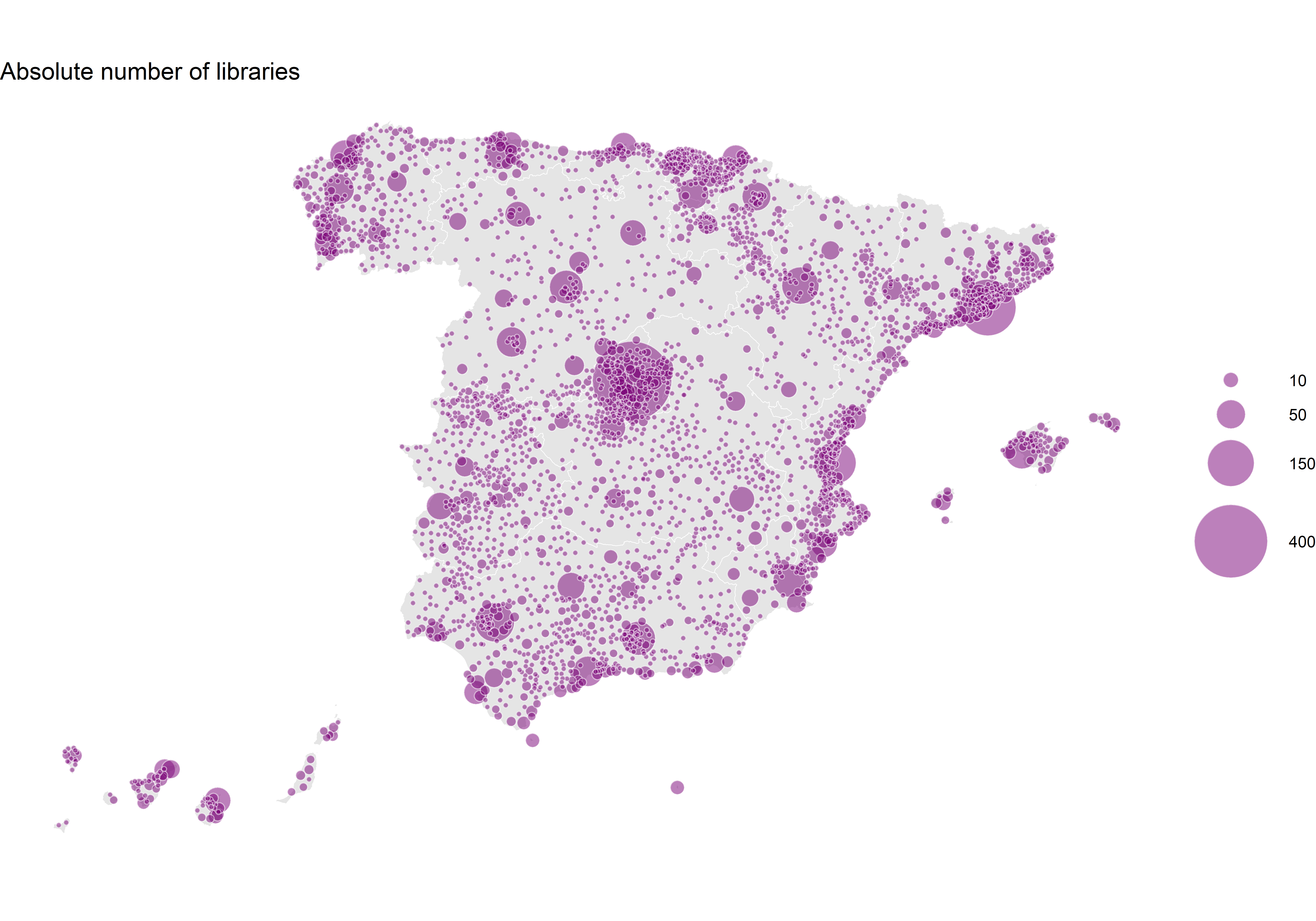
To create a proportional symbol map, we simply use the centroid of the municipality for the location. It is important to order the observations from highest to lowest, which ensures that the smaller circles are drawn on top of the larger ones.
In ggplot2, we use geom_sf() for the vector data and indicate size with the column n. Additionally, we set the size range with scale_size() and specify the breaks in the legend. We are also making a few small aesthetic changes.
m1 <- st_centroid(mun) |> arrange(-n)

p1 <- ggplot() +
  geom_sf(data = ccaa, fill = "grey90", colour = "white") +
  geom_sf(
    data = m1,
    aes(size = n),
    alpha = .5, shape = 21, fill = "#7a0177", colour = "white"
  ) +
  scale_size(range = c(1, 20), breaks = c(10, 50, 150, 400)) +
  labs(size = NULL, title = "Absolute number of libraries") +
  theme_void()
p1
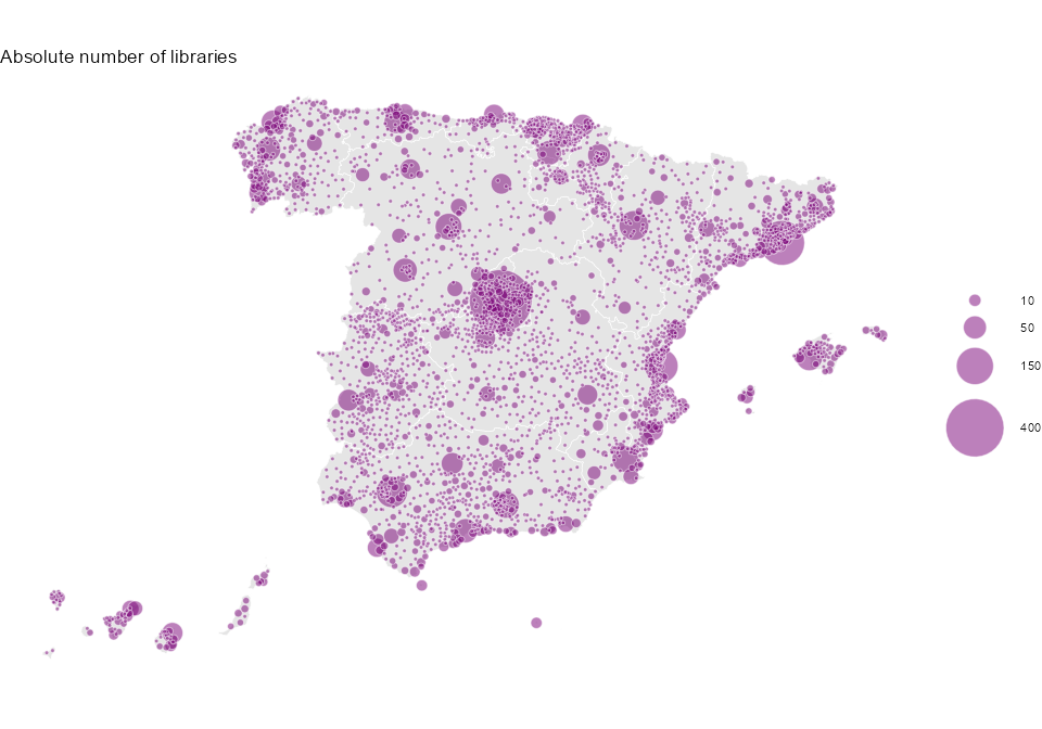
This map clearly resembles the one in the national atlas. Big cities, such as Madrid, Barcelona or Valencia, are highlighted.
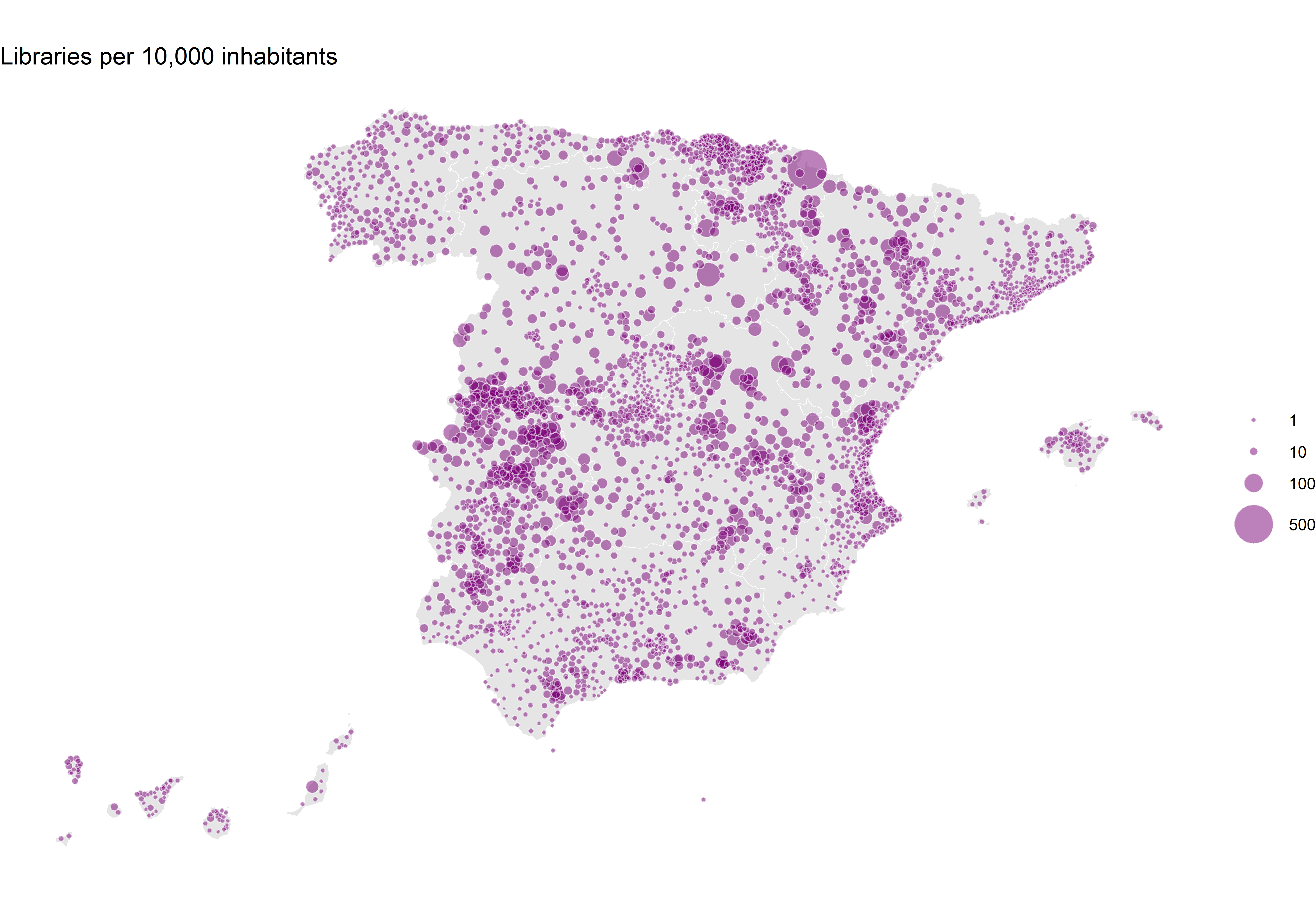
But what would we see if we normalize the variable?
To do this, we must first join the population data and calculate the rate.
m2 <- st_centroid(mun) |>
  left_join(pob_mun) |>
  mutate(norm_pob = n * 10000 / total) |>
  arrange(-norm_pob)

select(m2, n, total:norm_pob)
Now we simply repeat the same map using the norm_pob column.
p2 <- ggplot() +
  geom_sf(data = ccaa, fill = "grey90", colour = "white") +
  geom_sf(
    data = m2,
    aes(size = norm_pob),
    alpha = .5, shape = 21, fill = "#7a0177", colour = "white"
  ) +
  scale_size(range = c(.5, 10), breaks = c(1, 10, 100, 500)) +
  labs(size = NULL, title = "Libraries per 10,000 inhabitants") +
  theme_void()
p2
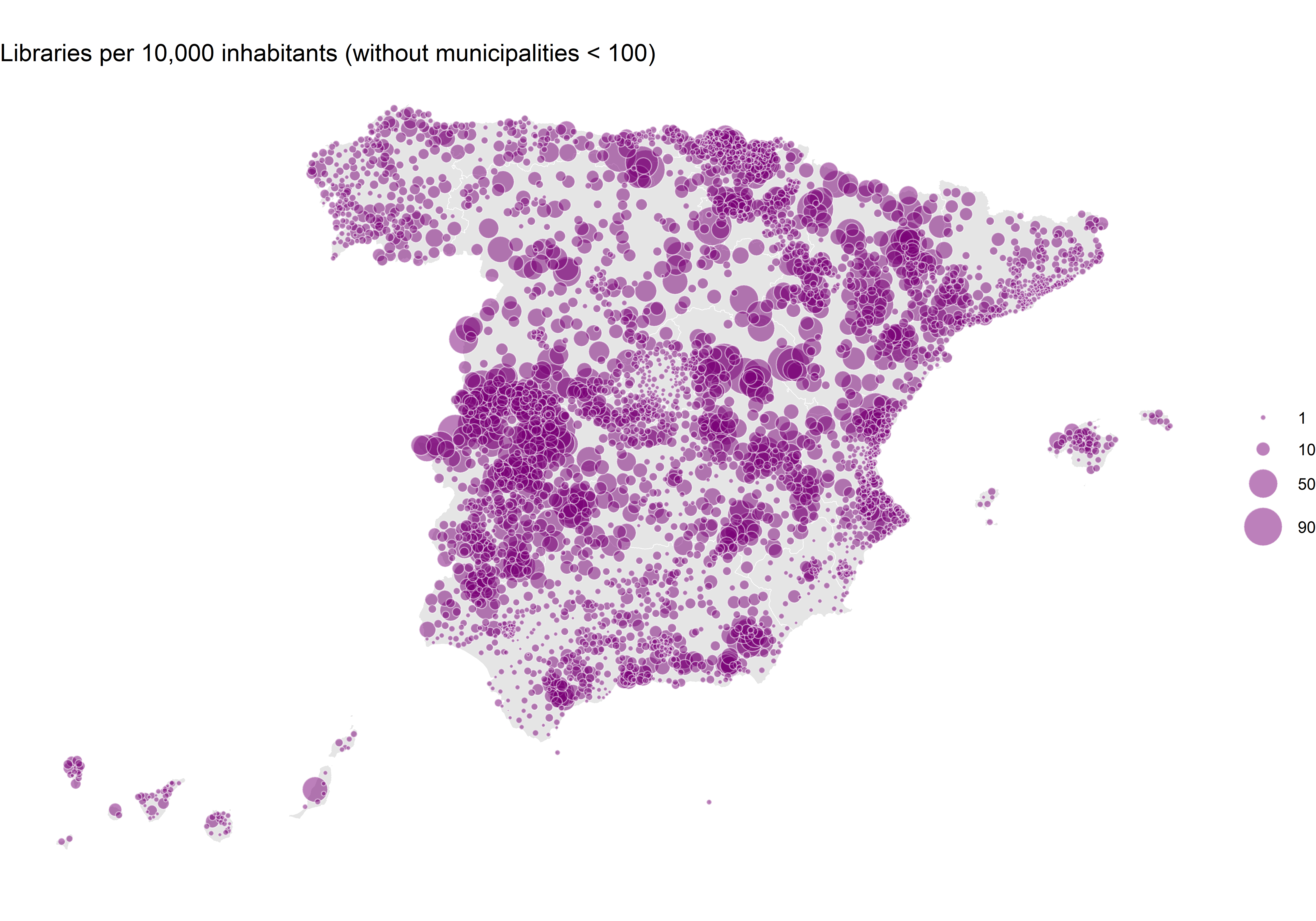
This map now tells a completely different story. We see a high number of libraries per inhabitant in certain regions, while others are more homogeneous with a consistently low number of libraries. However, there are also impossible values that stand out. For example, in the north, Roncesvalles reaches 526 libraries per 10,000 inhabitants! That can’t be right, can it? This issue is caused by the very small municipalities. In this case, there is one library for every 19 inhabitants. In any case, what is also noticeable is that there are significantly fewer libraries per inhabitant in major cities like Madrid and Barcelona, with only 1 library per 10,000 inhabitants. It is not easy to find a multiplier that works uniformly to reflect both small and large municipalities.
To solve the problem of small municipalities, one possible good strategy would be to exclude all those with less than 100 inhabitants. It can even help in reducing overlapping.
p3 <- ggplot() +
  geom_sf(data = ccaa, fill = "grey90", colour = "white") +
  geom_sf(
    data = filter(m2, total > 100),
    aes(size = norm_pob),
    alpha = .5, shape = 21, fill = "#7a0177", colour = "white"
  ) +
  scale_size(range = c(.1, 10), breaks = c(1, 10, 50, 90)) +
  labs(size = NULL, title = "Libraries per 10,000 inhabitants (without municipalities < 100)") +
  theme_void()

p3
Finally, we create a comparison with the patchwork grammar.
p1 + p2 + p3 & theme(plot.title = element_text(size = 20, hjust = .5),
                    legend.text = element_text(size = 12))
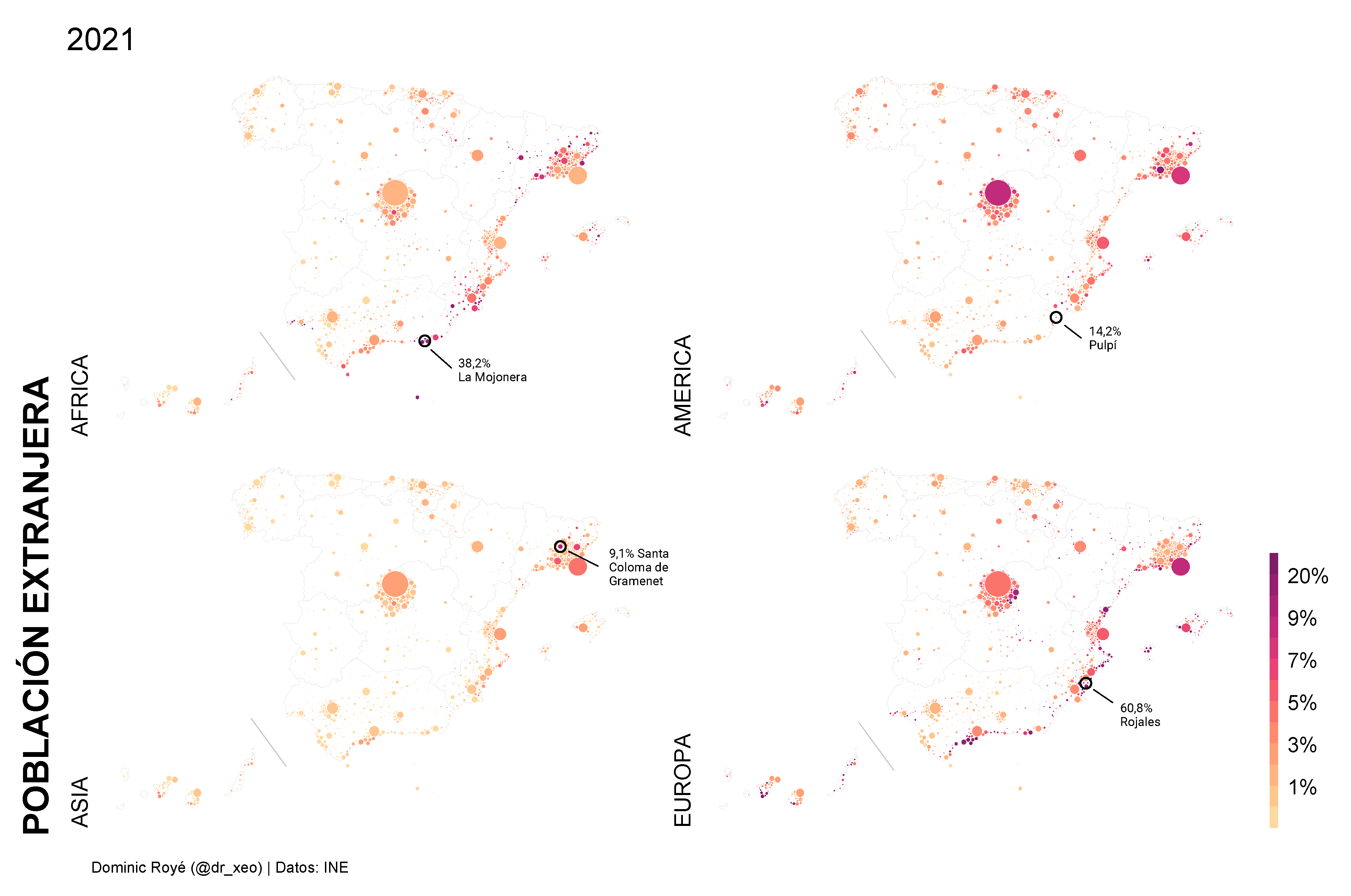
Different ways of telling different stories! A completely different question is how much the overlapping of circles prevents us from reading the map accurately. For instance, we could use a Dorling cartogram for the population and use color to show the number of libraries. Below, you see an example with the foreign population by origin. The R Code for this I will post another time.
Footnotes
Include also population data.↩︎
