Calculating the distance to the sea in R

The distance to the sea is a fundamental variable in geography, especially relevant when it comes to modeling. For example, in interpolations of air temperature, the distance to the sea is usually used as a predictor variable, since there is a casual relationship between the two that explains the spatial variation. How can we estimate the (shortest) distance to the coast in R?

Packages

In this post we will use the following libraries:

Library	Description
tidyverse	Collection of packages (visualization, manipulation): ggplot2, dplyr, etc.
sf	Simple Feature: import, export and manipulate vector data
raster	Import, export and manipulate raster
rnaturalearth	Set of vector maps ‘natural earth’
RColorBrewer	Color palettes

#install the libraries if necessary
if(!require("tidyverse")) install.packages("tidyverse")
if(!require("sf")) install.packages("sf")
if(!require("raster")) install.packages("raster")
if(!require("giscoR")) install.packages("giscoR")

#packages
library(giscoR)
library(sf)
library(raster)
library(tidyverse)
library(RColorBrewer)

The coast of Iceland as an example

Our example in this post will be Iceland, and, as it is an island territory it will facilitate the tutorial showing the process in a simple manner. The giscoR package allows you to import the boundaries of countries (with different administrative levels) from around the world. The gisco_get_countries( ) function imports the country boundaries. In this case we indicate with the argument scale the resolution (3, 10, 60m), with country we can indicate the specific country or contries of interest.

world <- gisco_get_countries(resolution = "60") #world map with 50m resolution

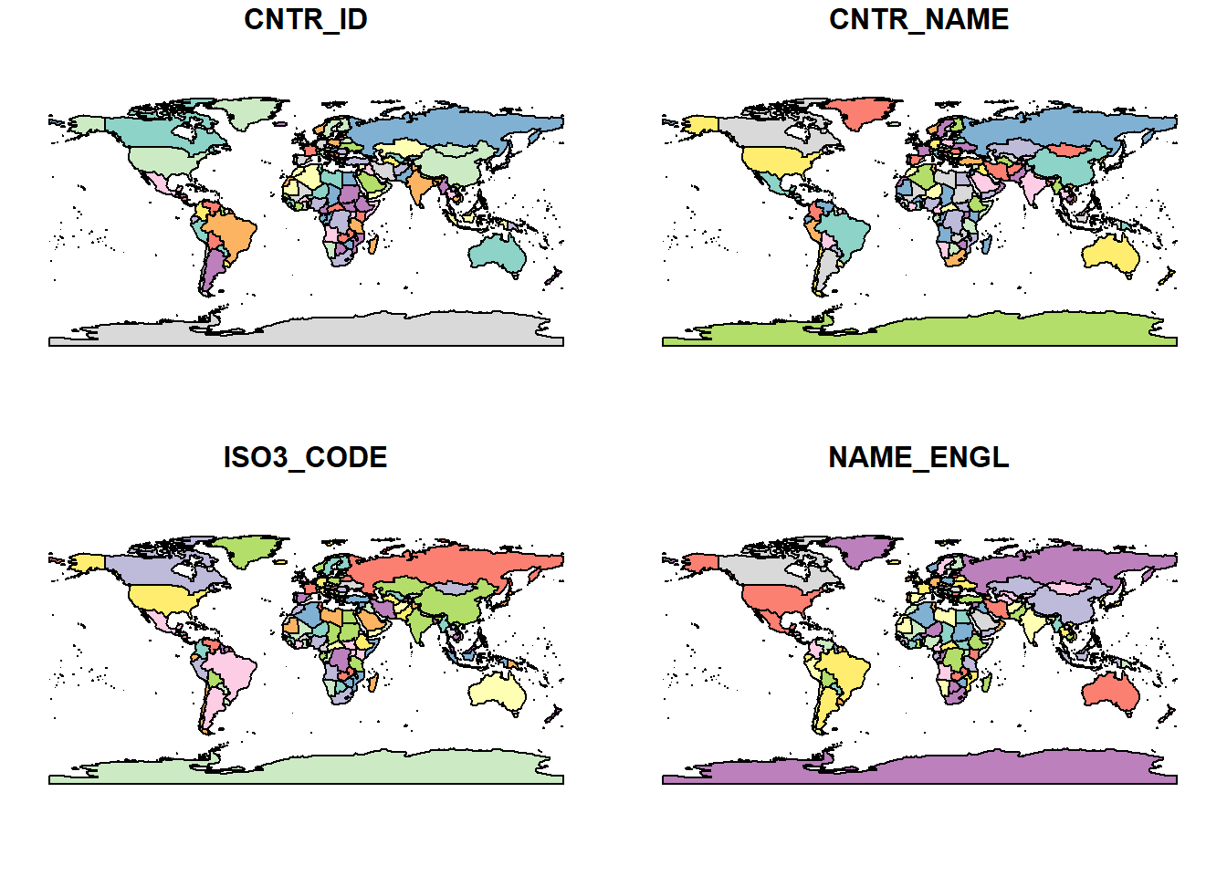
plot(world) #sp class by default

#import the limits of Iceland
iceland <- gisco_get_countries(resolution = "10", country = "Iceland")

#info of our spatial vector object
iceland

Simple feature collection with 1 feature and 4 fields
Geometry type: MULTIPOLYGON
Dimension:     XY
Bounding box:  xmin: -24.31733 ymin: 63.40177 xmax: -13.55855 ymax: 66.58179
Geodetic CRS:  WGS 84
  CNTR_NAME ISO3_CODE CNTR_ID NAME_ENGL                       geometry
1    Ísland       ISL      IS   Iceland MULTIPOLYGON (((-15.78316 6...

#here Iceland
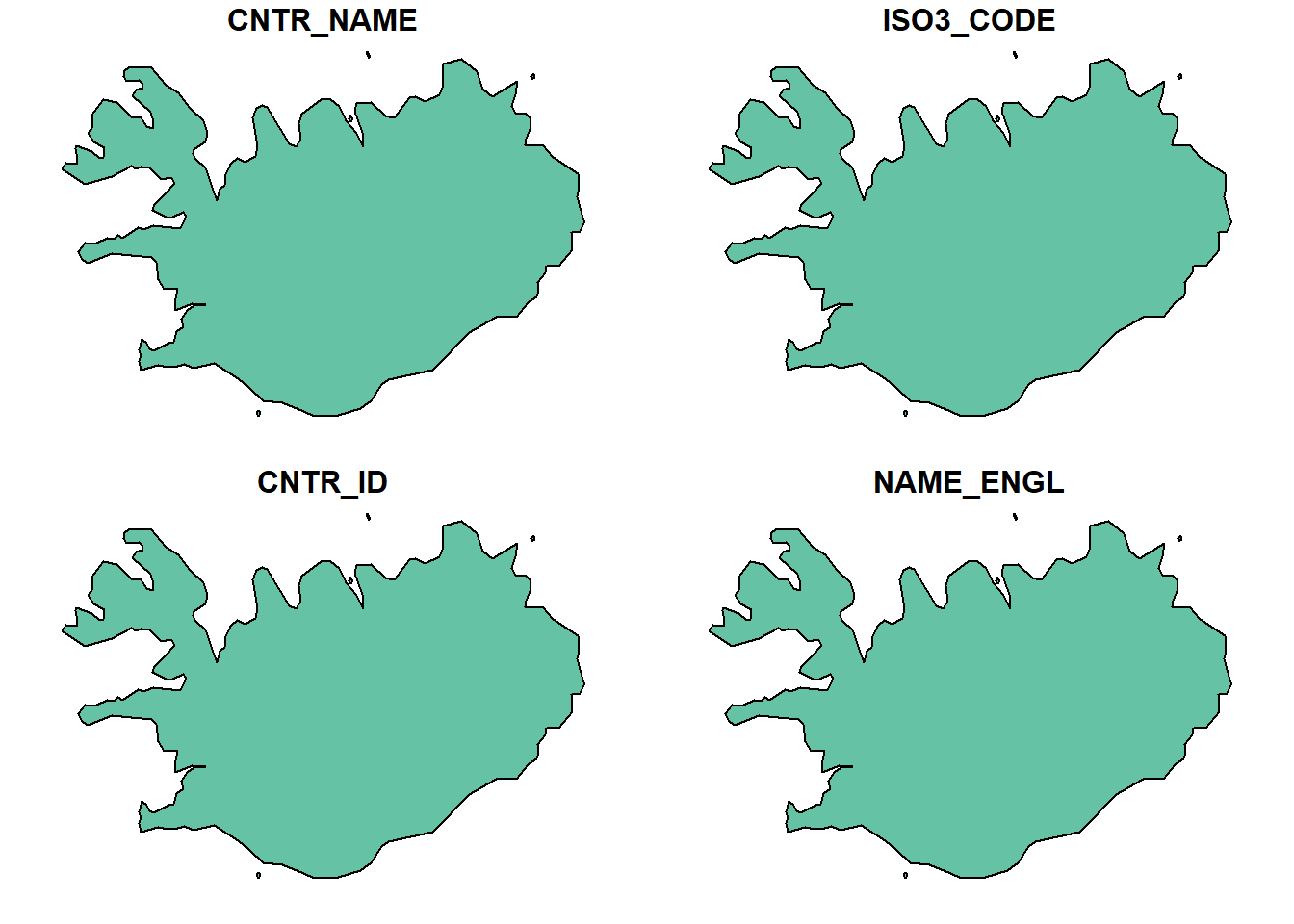
plot(iceland)

By default, the plot( ) function with the class sf creates as many facets of the map as there are variables in it. To limit this behavior we can use either a variable name plot(iceland["admin"]) or the limit argument plot(iceland, max.plot = 1). With the argument max.plot = 1 the function uses the first available variable of the map.

In addition, we see in the information of the object sf that the projection is WGS84 with decimal degrees (EPSG code: 4326). For the calculation of distances it is more convenient to use meters instead of degrees. Because of this, the first thing we do is to transform the map of Iceland to UTM Zone 27 (EPSG code: 3055). More information about EPSG and projections here. For that purpose, we use the st_transform( ) function. We simply indicate the map and the EPSG code.

#transform to UTM
iceland <- st_transform(iceland, 3055)

Create a fishnet of points

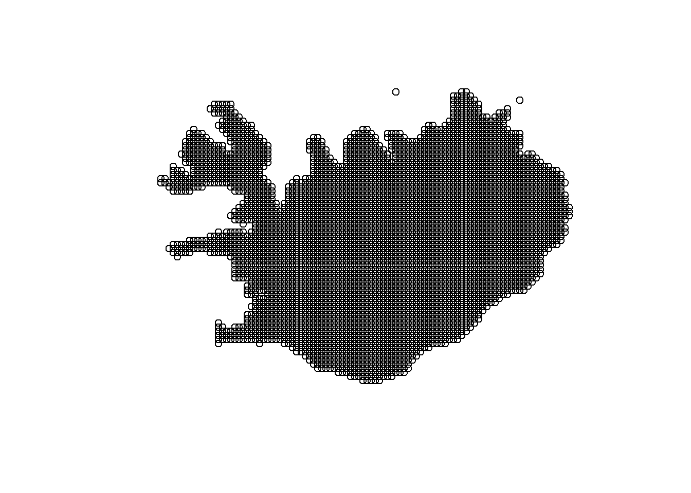
We still need the points where we want to know the distance. In our case it will be a regular fishnet of points in Iceland with a resolution of 5km. We do this with the function st_make_grid( ), indicating the resolution in the unit of the coordinate system (meters in our case) with the argument cellsize, and what geometry we would like to create what (polygons, centers or corners).

#create the fishnet
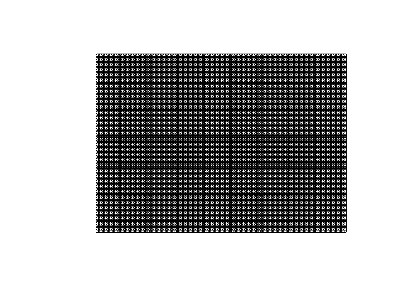
grid <- st_make_grid(iceland, cellsize = 5000, what = "centers")

#our fishnet with the extension of Iceland
plot(grid)

#only extract the points in the limits of Iceland
grid <- st_intersection(grid, iceland)   

#our fishnet now
plot(grid)

Calculating the distance

To estimate the distance we use the st_distance( ) function that returns a vector of distances for all our points in the fishnet. But first it is necessary to transform the map of Iceland from a polygon shape (MULTIPOLYGON) to a line (MULTILINESTRING). More details with ?st_cast.

#transform Iceland from polygon shape to line
iceland <- st_cast(iceland, "MULTILINESTRING")

#calculation of the distance between the coast and our points
dist <- st_distance(iceland, grid)

#distance with unit in meters
head(dist[1,])

Units: [m]
[1] 1345.506 1330.656 1315.806 1300.956 1286.106 1101.029

Plotting the calculated distance

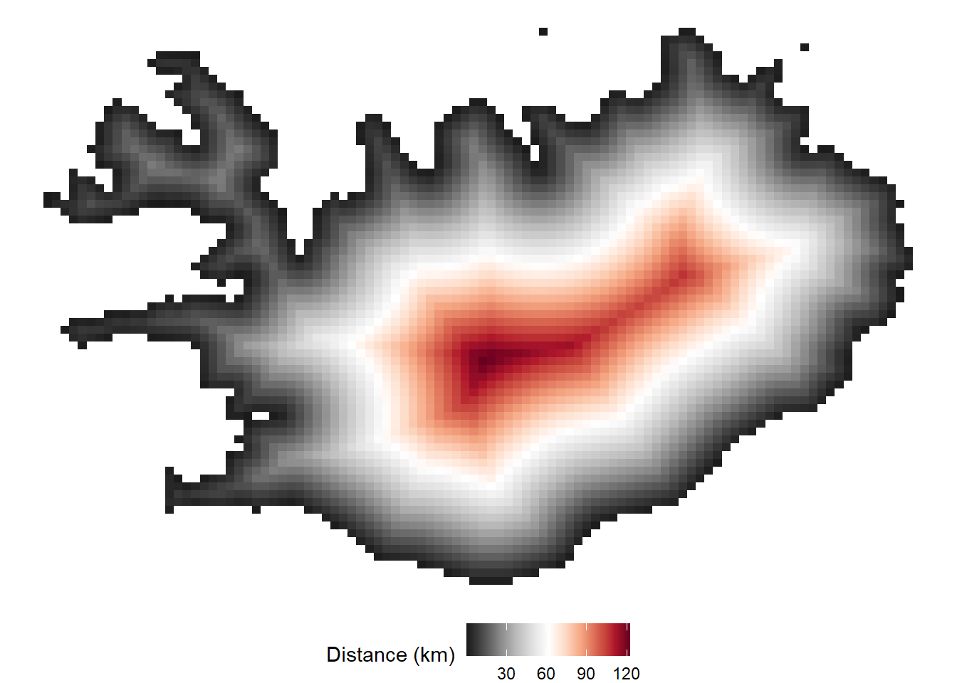
Once obtained the distance for our points, we can combine them with the coordinates and plot them in ggplot2. For this, we create a data.frame. The object dist is a matrix of one column, so we have to convert it to a vector with the function as.vector( ). In addition, we divide by 1000 to convert the distance in meters to km. The st_coordinates( ) function extracts the coordinates of our points. For the final visualization we use a vector of colors with the RdGy palette (more here).

#create a data.frame with the distance and the coordinates of the points
df <- data.frame(dist = as.vector(dist)/1000,
                    st_coordinates(grid))

#structure
str(df)

'data.frame':   4090 obs. of  3 variables:
 $ dist: num  1.35 1.33 1.32 1.3 1.29 ...
 $ X   : num  594378 599378 604378 609378 614378 ...
 $ Y   : num  7033908 7033908 7033908 7033908 7033908 ...

#colors 
col_dist <- brewer.pal(11, "RdGy")


ggplot(df, aes(X, Y, fill = dist))+ #variables
         geom_tile()+ #geometry
           scale_fill_gradientn(colours = rev(col_dist))+ #colors for plotting the distance
             labs(fill = "Distance (km)")+ #legend name
             theme_void()+ #map theme
              theme(legend.position = "bottom") #legend position

Export the distance as a raster

To be able to export the estimated distance to the sea of Iceland, we need to use the rasterize( ) function of the library raster.

1. First, it is necessary to create an empty raster. In this raster we have to indicate the resolution, in our case it is of 5000m, the projection and the extension of the raster.

   1. We can extract the projection from the information of the map of Iceland.

   2. The extension can be extracted from our grid points with the function extent( ). However, this last function needs the class sp, so we pass the object grid in sf format, only for this time, to the class sp using the function as( ) and the argument “Spatial”.

2. In addition to the above, the data.frame df, that we created earlier, has to be converted into the sf class. Therefore, we apply the function st_as_sf( ) with the argument coords indicating the names of the coordinates. Additionally, we also define the coordinate system that we know.

#get the extension
ext <- extent(as(grid, "Spatial"))

#extent object
ext

class      : Extent 
xmin       : 349377.7 
xmax       : 844377.7 
ymin       : 7033908 
ymax       : 7383908 

#raster destination
r <- raster(resolution = 5000, ext = ext, crs = "+proj=utm +zone=27 +ellps=intl +towgs84=-73,47,-83,0,0,0,0 +units=m +no_defs")

#convert the points to a spatial object class sf
dist_sf <- st_as_sf(df, coords = c("X", "Y")) %>%
                      st_set_crs(3055)

#create the distance raster
dist_raster <- rasterize(dist_sf, r, "dist", fun = mean)

#raster
dist_raster

class      : RasterLayer 
dimensions : 70, 99, 6930  (nrow, ncol, ncell)
resolution : 5000, 5000  (x, y)
extent     : 349377.7, 844377.7, 7033908, 7383908  (xmin, xmax, ymin, ymax)
crs        : +proj=utm +zone=27 +ellps=intl +towgs84=-73,47,-83,0,0,0,0 +units=m +no_defs 
source     : memory
names      : layer 
values     : 0.00274077, 122.3031  (min, max)

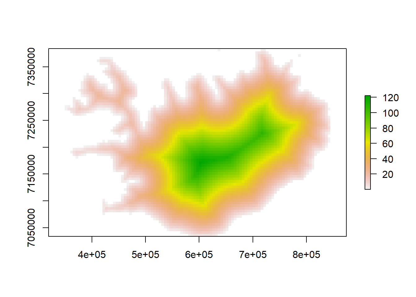
#plot the raster
plot(dist_raster)

#export the raster
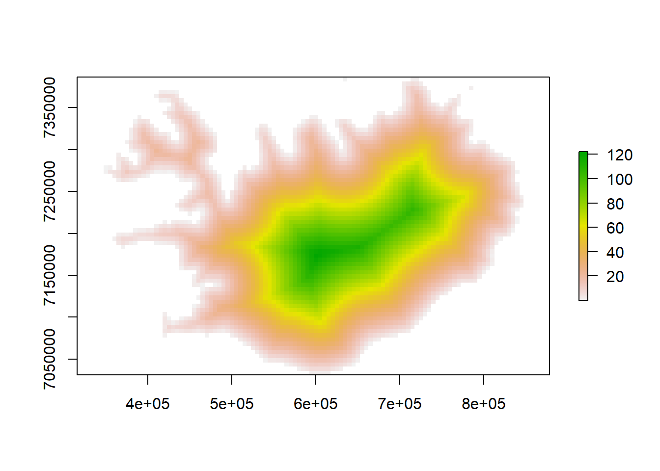
writeRaster(dist_raster, file = "dist_islandia.tif", format = "GTiff", overwrite = TRUE)

The rasterize( ) function is designed to create rasters from an irregular grid. In case we have a regular grid, like this one, we can use an easier alternative way. The rasterFromXYZ( ) function converts a data.frame with longitude, latitude and the variable Z into a raster object. It is important that the order should be longitude, latitude, variables.

r <- rasterFromXYZ(df[, c(2:3, 1)], crs = "+proj=utm +zone=27 +ellps=intl +towgs84=-73,47,-83,0,0,0,0 +units=m +no_defs")

plot(r)

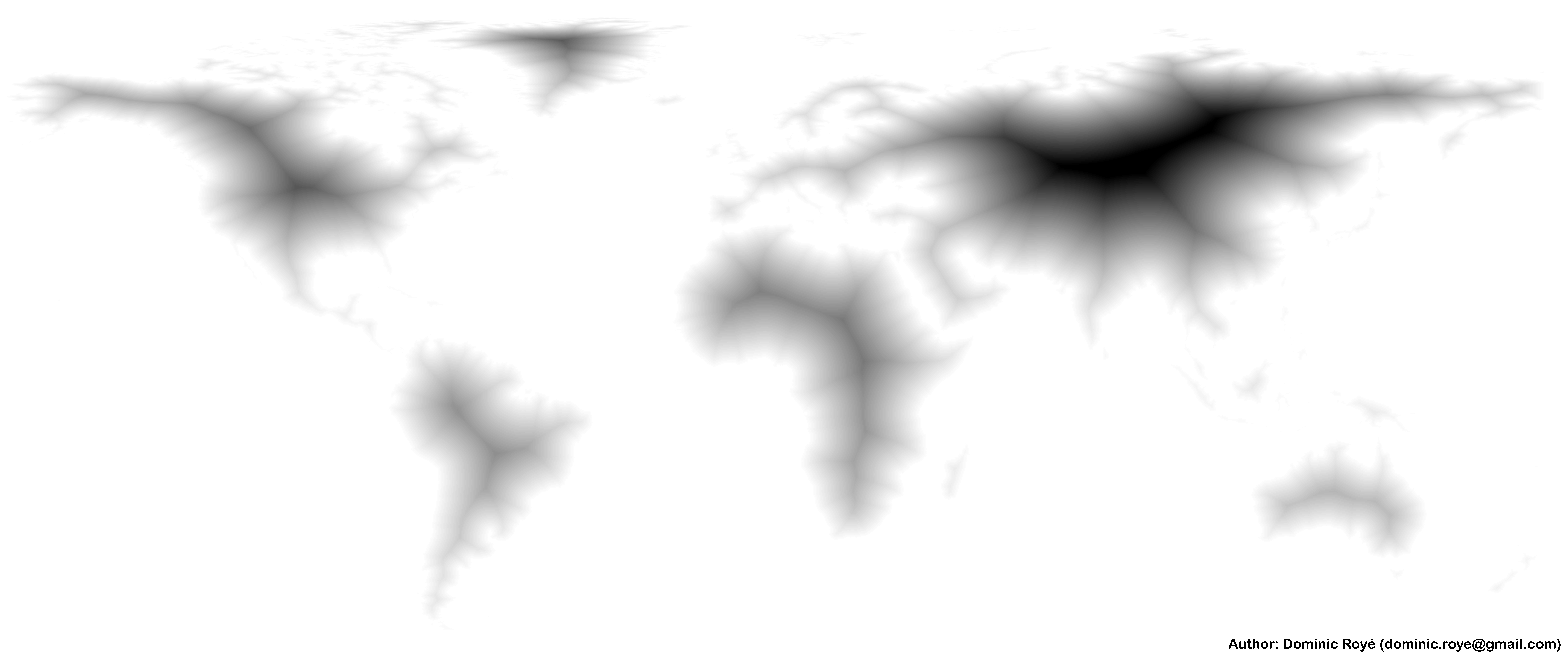
With the calculation of distance we can create art, as seen in the header of this post, which includes a world map only with the distance to the sea of all continents. A different perspective to our world (here more (spanish)) .