pkgs <- c("terra","sf","tidyverse","fs","mgcv","elevatr","mapSpain", "patchwork", "tidyterra")
for(p in pkgs) if(!require(p, character.only = TRUE)) install.packages(p)

library(terra)
library(sf)
library(tidyverse)
library(fs)
library(mgcv)
library(elevatr)
library(mapSpain)
library(tidyterra)
library(patchwork)Downscaling solar radiation in the Canary Islands with GAM
Spatial analysis
Geostatistics
R:Advanced
GAM
R
terra
downscaling
I’ve been meaning to write a post on how we can push interpolation and downscaling— beyond the usual tools like linear regression or kriging when dealing with climate data. This post illustrates a statistical downscaling workflow for monthly radiation over the Canary Islands using a Generalized Additive Model (GAM). We start from a coarse ~5km signal, learn its relationship with topography and MODIS cloudiness, and then predict to a finer 1km grid. The approach is intentionally lightweight: a single-month example (January) and a compact set of predictors.
The Canary Islands offer a particularly compelling test case for downscaling because of their extremely complex orography and sharp local climate gradients. With steep volcanic relief rising from sea level to over 3,000m in very short horizontal distances, conditions can change dramatically within a few kilometres. However, the native Meteosat resolution of around 5km smooths out much of this spatial variability, blending together zones that in reality experience very different levels of cloudiness and thus solar radiation.
Tip
GAMs are flexible enough to capture non-linear effects and interactions (e.g., cloudiness × elevation) while remaining interpretable thanks to smooth terms.
Packages
| Package | Description |
|---|---|
| terra | The modern standard for spatial data analysis, providing high-performance methods for manipulating and modeling raster and vector data. |
| sf | Provides “Simple Features” support for R, serving as the core package for handling and transforming vector-based geographic data (points, lines, polygons). |
| tidyverse | A foundational collection of packages (visualization, manipulation): ggplot2, dplyr, purrr, etc., designed for cohesive data science workflows. |
| fs | Offers a cross-platform, uniform interface for file system operations, making path and file management more robust and readable. |
| mgcv | The industry-standard library for Generalized Additive Models (GAMs). |
| elevatr | Provides access to global elevation data APIs, simplifying the automated download of Digital Elevation Models (DEM) for any study area. |
| mapSpain | A specialized tool for downloading high-quality administrative boundaries and cartographic data for Spain at multiple scales. |
| tidyterra | Bridges the gap between terra and ggplot2, allowing for the direct and efficient visualization of SpatRaster and SpatVector objects. |
| patchwork | A powerful layout tool that makes it incredibly simple to combine separate ggplot objects into a single, cohesive, publication-ready figure. |
Study area and inputs
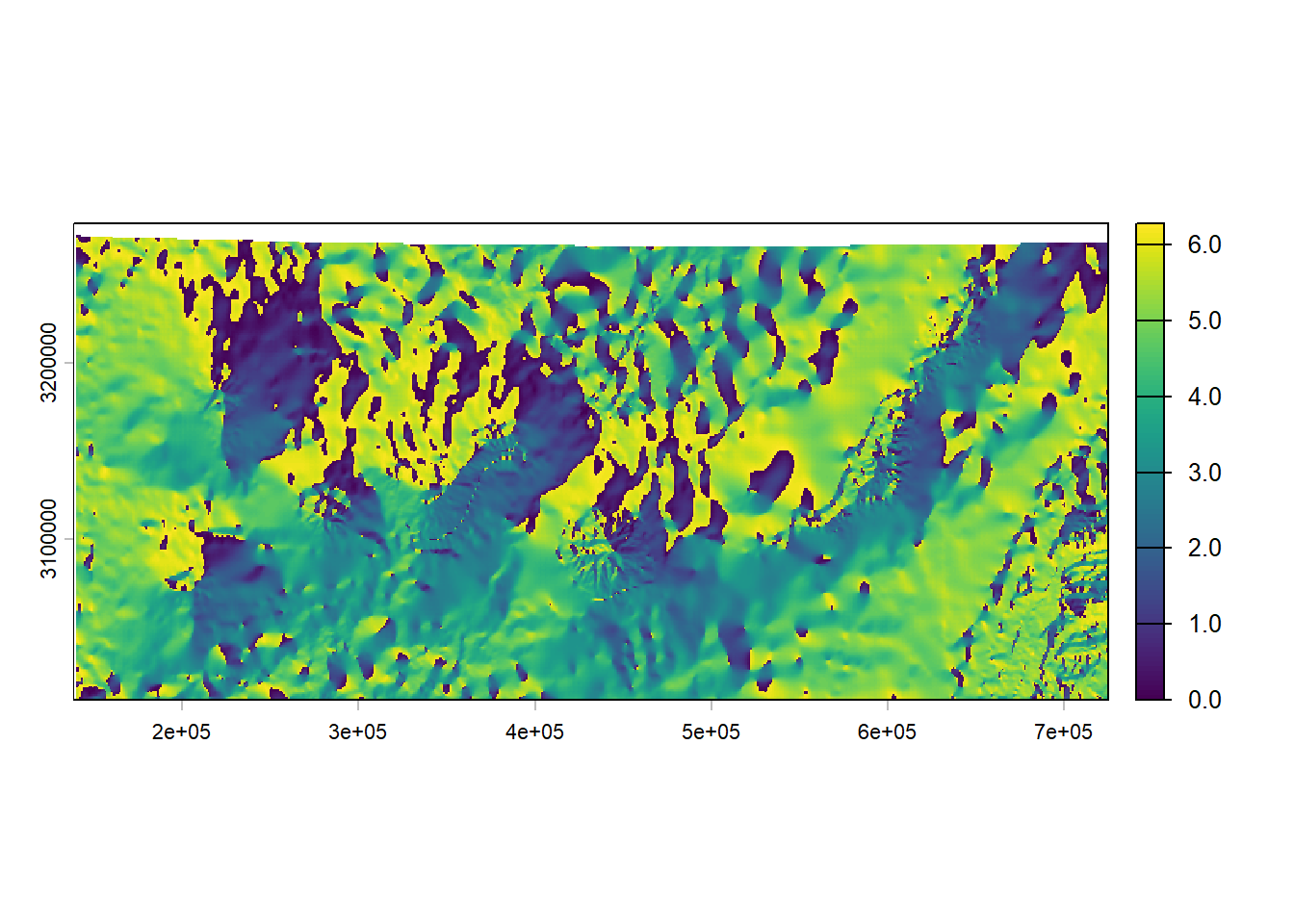
We import the Canary geometry with names for each Island, transform it to EPSG:4083, and load: - Cloudiness (MODIS proxy, see below) at ~1km. - Total sunhours (coarse, ~5km) for January 2026 (accessible via EUMETSAT - CMSAF) - Elevation from elevatr package to derive slope and aspect at both 5km and 1km.
To derive the monthly cloudiness climatology from MODIS, I combined the Terra (morning) and Aqua (afternoon) surface reflectance collections in Google Earth Engine (script) and extracted a simple cloud-state indicator from the state_1km QA band. Pixels flagged as clear, mixed, or cloudy were converted to continuous values (0, 0.5, 1), while missing or masked states were excluded. The result is a 1‑km image summarising the average monthly cloud conditions over the region for January 2026.
Note
You can download the used datasets here.
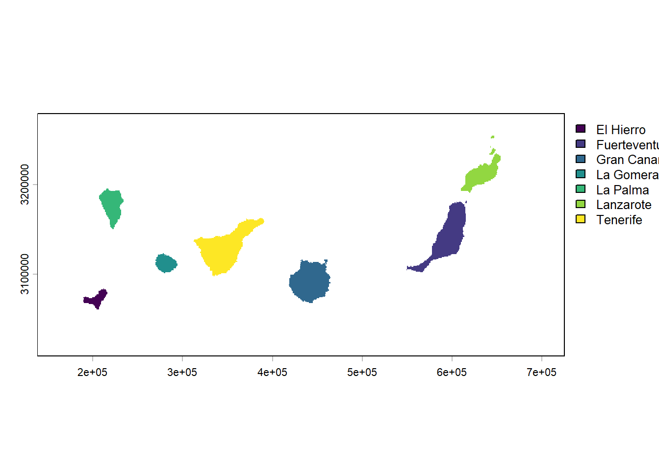
# Canary Islands geometry
can <- st_read("islas_20170101_generalizada.json")
Reading layer `islas_20170101_generalizada' from data source
`C:\Users\xeo19\Nextcloud\New web\blog\canary-gam-downscaling\islas_20170101_generalizada.json'
using driver `GeoJSON'
Simple feature collection with 7 features and 15 fields
Geometry type: MULTIPOLYGON
Dimension: XY
Bounding box: xmin: -18.16083 ymin: 27.63773 xmax: -13.33512 ymax: 29.41606
Geodetic CRS: WGS 84can <- st_transform(can, 4083)
# MODIS ~1 km cloudiness
modis_1km <- rast("cloud_jan_26.tif") |> project("EPSG:4083")
plot(modis_1km) # rate 0 to 1 = (0-100%)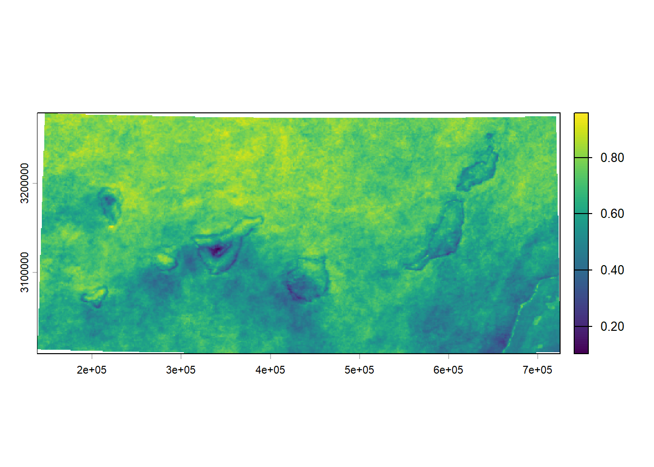
# resample cloudiness at 4 km
modis_4km <- resample(modis_1km, sol_4km, method = "bilinear")
isla_rast_4km <- rasterize(can, rast(sol_4km), field = "etiqueta")
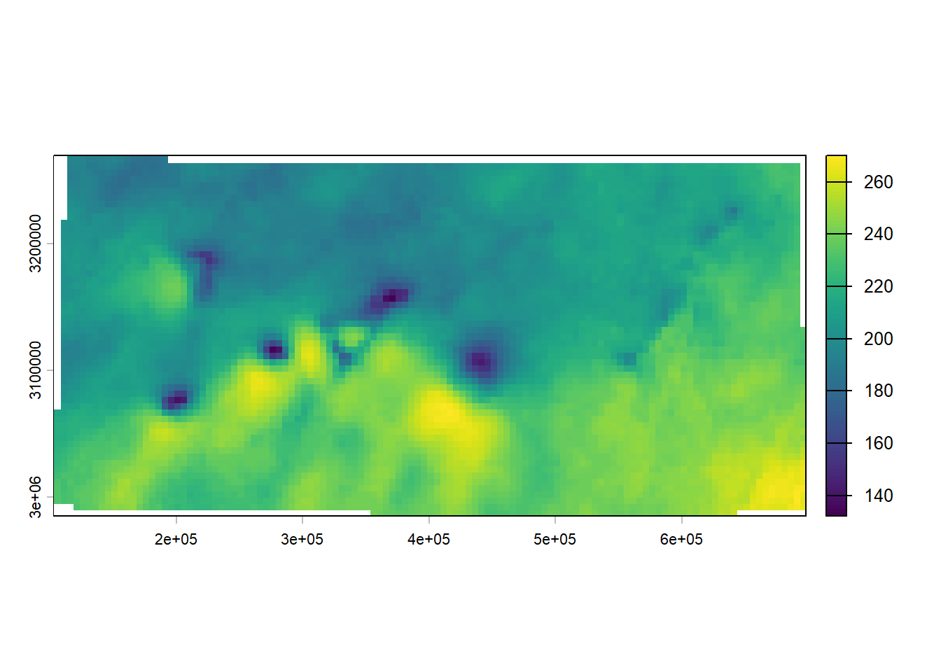
# Elevation and terrain metrics at both resolutions
elev <- get_elev_raster(modis_4km, z = 7) |> rast() |> project("EPSG:4083")
elev_4km <- resample(elev, sol_4km, method = "bilinear")
elev_1km <- resample(elev, modis_1km, method = "bilinear")
plot(elev_1km)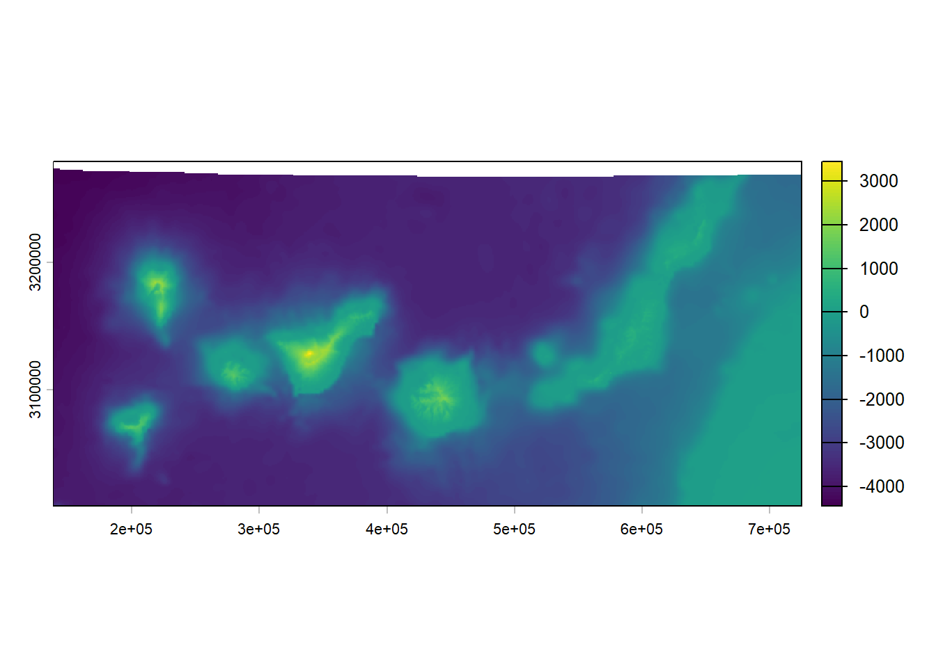
Tip
Computing slope or aspect directly at 5km loses important terrain information because the coarse resolution smooths out real topographic variability. By deriving these metrics at 1km first, you preserve the finer‑scale gradients before aggregating them.
For a discrete variable like the islands, rasterizing directly at 5km is appropriate because the categories should not be smoothed or interpolated. Resampling a discrete class would mix labels, so rasterization at the target resolution preserves the original categorical boundaries.
Build modelling tables
We assemble a training table at 5km (response + predictors) and a prediction table at 1km (predictors only). For convenience we mask to the islands polygon.
# Training stack (4 km)
lay <- c(sol_4km, modis_4km, elev_4km, sl_4km, asp_4km, isla_rast_4km)
lay <- mask(lay, can)

df <- as.data.frame(lay, xy = TRUE)
names(df) <- c("x","y","sunhr","cloud","elev","sl","asp","isl")

df <- mutate(df, sin_asp = sin(asp), cos_asp = cos(asp))

# Prediction (1 km)
lay_pred <- c(modis_1km, elev_1km, sl_1km, asp_1km, isla_rast_1km)
lay_pred <- mask(lay_pred, can)

df_pred <- as.data.frame(lay_pred, xy = TRUE, na.rm = TRUE)
names(df_pred) <- c("x","y","cloud","elev","sl","asp", "isl")

df_pred <- mutate(df_pred, sin_asp = sin(asp), cos_asp = cos(asp))

glimpse(df)
Rows: 448
Columns: 10
$ x <dbl> 640977.3, 645982.2, 640977.3, 645982.2, 640977.3, 645982.2, 65…
$ y <dbl> 3252540, 3252540, 3242530, 3242530, 3237525, 3237525, 3237525,…
$ sunhr <dbl> 21.35235, 21.72177, 21.32614, 21.52760, 21.09057, 21.19915, 21…
$ cloud <dbl> 0.6225122, 0.5350854, 0.6715685, 0.6021773, 0.6255413, 0.58443…
$ elev <dbl> -208.0254974, -6.7074027, -87.0284271, -8.0537682, -37.6034660…
$ sl <dbl> 6.6919975, 2.1266482, 2.5276296, 0.8959233, 1.6019516, 1.79989…
$ asp <dbl> 4.478906, 2.133024, 4.848343, 2.692572, 5.041506, 2.693937, 1.…
$ isl <fct> NA, Lanzarote, NA, NA, NA, Lanzarote, NA, NA, NA, NA, Lanzarot…
$ sin_asp <dbl> -0.972866485, 0.846069840, -0.990772493, 0.434083800, -0.94632…
$ cos_asp <dbl> -0.23136724, -0.53307206, 0.13553549, -0.90087250, 0.32320739,…Model: GAM for spatial downscaling
In this section we progressively build the downscaling model, starting from a very simple baseline and incrementally adding predictors. This step‑by‑step approach helps illustrate how each component contributes to recovering the spatial variability that the native 5km Meteosat resolution cannot resolve over the highly complex orography of the Canary Islands.
To be brief about GAMs. The s() function is the “smoother” in a GAM. It tells the model to find a flexible curve that actually follows the pattern of your data. It uses a penalty system to automatically find the perfect balance between following the data and staying smooth. It decides the shape for you. The bs argument defines the type of curve used to build that shape. Knots are the specific anchor points along the data where the spline is allowed to bend and change its shape. They act like joints or hinges connecting the different polynomial pieces that make up the curve.
| Argument | Basis Type | Key Feature |
|---|---|---|
| tp | Thin Plate | Default. Optimal smoothing; no manual knots |
| cr | Cubic Natural | Linear at edges |
| cc | Cyclic Connected | End point matches start point |
| bs | B-spline Modular | Uses standard B-spline bases |
| ps | P-spline Penalized | Discrete penalty on wiggliness |
| so | Soap Film Bounded | Does not “leak” over boundaries |
| sos | Sphere Global | Continuous across the globe |
| gp | Gaussian Process | Spatial. Based on point-to-point correlation |
Tip
The mgcv package has the bam() function for large datasets with the posibility of multiple CPU cores use (100k+ rows).
1. Baseline model: only spatial coordinates
We begin with the simplest possible GAM: a bivariate smooth over the coordinates. This model captures only broad spatial gradients and serves as a lower bound for performance. Think of these as our “foundation” before adding complex physical variables like cloud cover or elevation.
The first model is the simplest spatial approach. It treats the entire archipelago as a single continuous surface. It uses a bivariate smooth \(s(x, y)\) to find a general heat map of sunshine hours across all islands. But it assumes that the climate changes smoothly over the ocean between islands. In reality, a mountain in Tenerife creates a microclimate that has nothing to do with the flat plains of Lanzarote.
In the second model, we acknowledge that each island is its own “climatic universe.”
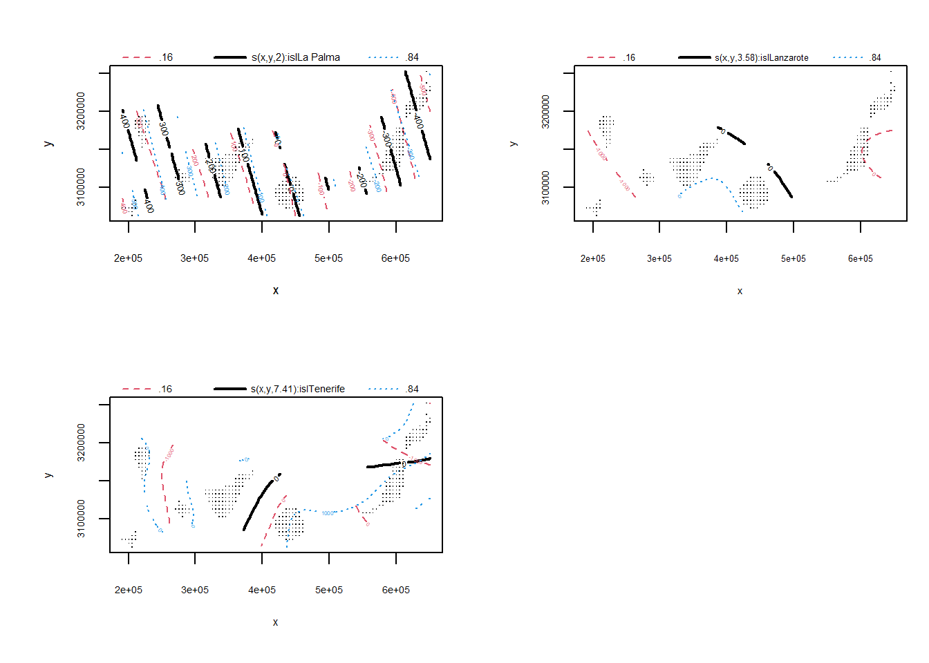
isl - 1: We remove the global intercept so each island gets its own baseline sunshine level.by = isl: give each island its own independent spatial surface \(s(x, y)\). This model respects the geographical fragmentation of the archipelago. It allows Tenerife to have a complex, curvy sunshine pattern while letting Lanzarote remain flatter and more uniform.
A critical decision in spatial GAMs is setting the basis dimension (\(k\)), which determines the maximum possible complexity of the smooth terms. For our island-specific model, we set \(k = 12\) for each \(s(x, y)\) term. In islands with dramatic orography like Tenerife or Gran Canaria, a low \(k\) (e.g., \(k=5\)) would “oversmooth” the results. One of the strengths of the mgcv framework is that \(k\) only sets the upper limit of complexity. The model uses penalized likelihood (REML) to dampen the smooth if it doesn’t find enough signal. We see this clearly in Lanzarote, where despite having \(k=12\) available, the model only used 2.00 DF, identifying the island’s sunshine pattern as a simple linear plane.
Family: gaussian
Link function: identity

Formula:
sunhr ~ s(x, y)

Parametric coefficients:
            Estimate Std. Error t value Pr(>|t|)
(Intercept) 20.46858    0.04876   419.8   <2e-16 ***
---
Signif. codes:  0 '***' 0.001 '**' 0.01 '*' 0.05 '.' 0.1 ' ' 1

Approximate significance of smooth terms:
         edf Ref.df     F p-value
s(x,y) 28.47  28.98 83.49  <2e-16 ***
---
Signif. codes:  0 '***' 0.001 '**' 0.01 '*' 0.05 '.' 0.1 ' ' 1

R-sq.(adj) =  0.843   Deviance explained = 85.3%
-REML =    720  Scale est. = 1.0651    n = 448
Family: gaussian
Link function: identity

Formula:
sunhr ~ isl - 1 + s(x, y, by = isl, k = 12)

Parametric coefficients:
                   Estimate Std. Error t value Pr(>|t|)
islEl Hierro     -1165.7825   500.6903  -2.328  0.02068 *
islFuerteventura    -0.1797    15.5364  -0.012  0.99078
islGran Canaria     78.7365    32.8479   2.397  0.01725 *
islLa Gomera       228.2052   324.5042   0.703  0.48255
islLa Palma        -18.2164     5.9190  -3.078  0.00232 **
islLanzarote       -23.6064    49.8294  -0.474  0.63609
islTenerife         44.0447    38.1691   1.154  0.24961
---
Signif. codes:  0 '***' 0.001 '**' 0.01 '*' 0.05 '.' 0.1 ' ' 1

Approximate significance of smooth terms:
                          edf Ref.df       F p-value
s(x,y):islEl Hierro     3.887  4.345  21.262 < 2e-16 ***
s(x,y):islFuerteventura 4.337  4.761  16.237 < 2e-16 ***
s(x,y):islGran Canaria  6.509  6.991 107.383 < 2e-16 ***
s(x,y):islLa Gomera     4.224  4.664  49.042 < 2e-16 ***
s(x,y):islLa Palma      2.000  2.000  27.397 < 2e-16 ***
s(x,y):islLanzarote     3.580  4.017   4.193 0.00333 **
s(x,y):islTenerife      7.411  7.922  93.978 < 2e-16 ***
---
Signif. codes:  0 '***' 0.001 '**' 0.01 '*' 0.05 '.' 0.1 ' ' 1

R-sq.(adj) =  0.904   Deviance explained = 91.6%
-REML = 366.37  Scale est. = 0.66764   n = 293
What to check
After running the initial spatial models, we can extract several key insights regarding the solar radiation field over the Canary Islands.
Effective Degrees of Freedom (EDF): In the global model (gam_base1), the smooth \(s(x,y)\) uses 28.4 EDF. This indicates a highly complex spatial surface where the model is forced to “stretch” a single spline across the entire archipelago to capture the sharp climatic contrasts between the islands.
Deviance Explained: The global baseline explains 85.3% of the deviance. While this is high for a starting point, moving to the island-specific model pushes this to 91.6%. This jump proves that the spatial organization of sunshine is not a single gradient, but a fragmented one dictated by the unique orography of each island.
Residual Variance (Scale Est.): The global model shows a scale estimate of 106.5. By simply allowing each island to have its own spatial trend, this variance drops drastically to 66.7. This significant reduction confirms that a large portion of the “error” in simpler models is actually just the ignored geographical boundaries between the islands.
Despite the high deviance explained (over 91% in the best spatial case), clear residual structure remains. The k-index and diagnostic checks signal that while \(x\) and \(y\) capture the “where,” they don’t capture the “why”. The model is still missing the fundamental physical drivers: the Sea of Clouds (interaction between clouds and elevation) and the terrain geometry (slope and aspect). These baselines confirm that while the 5km Meteosat signal has a strong spatial component, we need additional physical predictors to recover the finer-scale variability that coordinates alone cannot explain.
# some diagnostic plots and stats
plot(gam_base2, shade = TRUE, pages = 2)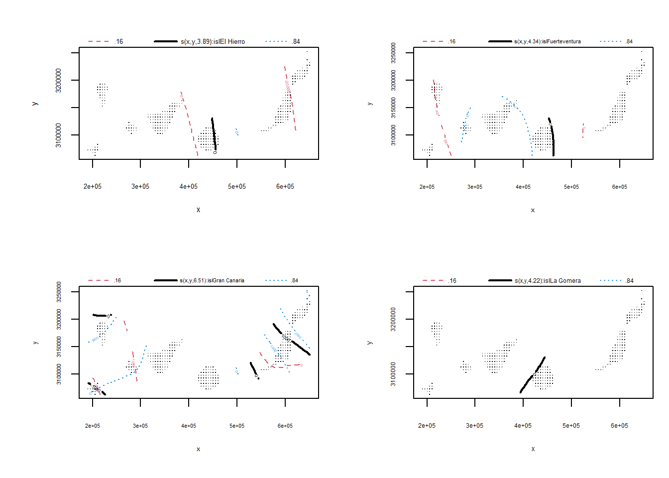
gam.check(gam_base2)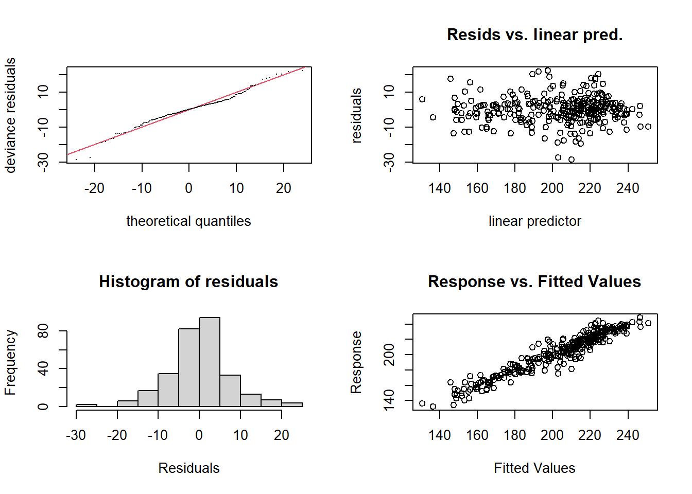
Method: REML   Optimizer: outer newton
full convergence after 16 iterations.
Gradient range [-1.674039e-06,1.145688e-05]
(score 366.369 & scale 0.6676394).
Hessian positive definite, eigenvalue range [1.674058e-06,136.123].
Model rank =  84 / 84

Basis dimension (k) checking results. Low p-value (k-index<1) may
indicate that k is too low, especially if edf is close to k'.

                           k'   edf k-index p-value
s(x,y):islEl Hierro     11.00  3.89     0.7  <2e-16 ***
s(x,y):islFuerteventura 11.00  4.34     0.7  <2e-16 ***
s(x,y):islGran Canaria  11.00  6.51     0.7  <2e-16 ***
s(x,y):islLa Gomera     11.00  4.22     0.7  <2e-16 ***
s(x,y):islLa Palma      11.00  2.00     0.7  <2e-16 ***
s(x,y):islLanzarote     11.00  3.58     0.7  <2e-16 ***
s(x,y):islTenerife      11.00  7.41     0.7  <2e-16 ***
---
Signif. codes:  0 '***' 0.001 '**' 0.01 '*' 0.05 '.' 0.1 ' ' 1
A low k-index (<1) means the basis dimension may be too low relative to the complexity of the underlying pattern. However, this is our baseline model, which intentionally uses only spatial coordinates. The fact that k appears borderline insufficient is actually expected, much of the spatial complexity is caused by other physical variables, not by pure spatial location.
2. Adding the first physical driver: cloudiness
Next we incorporate MODIS cloudiness, our likely strongest predictor for solar radiation from a physical point of view. This reveals how much fine‑scale variability can be explained by cloud patterns alone.
Family: gaussian
Link function: identity

Formula:
sunhr ~ isl - 1 + s(cloud) + s(x, y, by = isl, k = 12)

Parametric coefficients:
                  Estimate Std. Error t value Pr(>|t|)
islEl Hierro     -1131.966    470.849  -2.404   0.0169 *
islFuerteventura     1.660     12.930   0.128   0.8979
islGran Canaria     63.139     23.653   2.669   0.0081 **
islLa Gomera       151.912    244.769   0.621   0.5354
islLa Palma       -245.490    167.575  -1.465   0.1442
islLanzarote        -7.203     38.249  -0.188   0.8508
islTenerife         64.050     31.548   2.030   0.0434 *
---
Signif. codes:  0 '***' 0.001 '**' 0.01 '*' 0.05 '.' 0.1 ' ' 1

Approximate significance of smooth terms:
                          edf Ref.df      F  p-value
s(cloud)                2.827  3.627 28.591  < 2e-16 ***
s(x,y):islEl Hierro     4.082  4.545 16.003  < 2e-16 ***
s(x,y):islFuerteventura 4.309  4.730  7.167 1.43e-05 ***
s(x,y):islGran Canaria  6.276  6.875 61.240  < 2e-16 ***
s(x,y):islLa Gomera     4.114  4.571 37.703  < 2e-16 ***
s(x,y):islLa Palma      5.036  5.551  9.956  < 2e-16 ***
s(x,y):islLanzarote     3.448  3.890  6.286 0.000309 ***
s(x,y):islTenerife      7.356  7.870 37.097  < 2e-16 ***
---
Signif. codes:  0 '***' 0.001 '**' 0.01 '*' 0.05 '.' 0.1 ' ' 1

R-sq.(adj) =  0.932   Deviance explained = 94.2%
-REML = 325.12  Scale est. = 0.47106   n = 293
The output shows a clear improvement over the baseline model that used only the spatial coordinates. The smooth term for cloudiness now has an edf of 2.83, which, in this stage of the modeling, indicates that the relationship between cloud cover and sunshine hours has evolved beyond a simple linear fit. While GAMs are designed to capture complex non-linearities, the model now identifies that even at this 5km scale, the decrease in solar radiation follows a more nuanced, curved trajectory as cloudiness increases.
The high F-statistic (28.59) and the extremely small p-value (< 2e-16) confirm that cloudiness remains a dominant explanatory variable. Deviance explained remains high at 94.2%, while the residual variance (scale est.) is situated at 47.11. MODIS cloudiness carries information at 1km that Meteosat cannot resolve. Keep in mind that even when averaged to the 5km grid, cloudiness still helps distinguish areas that receive more or less solar radiation. However, because cloudiness alone does not yet encode elevation, slope, or exposure effects, the spatial smooths (\(s(x,y):isl\)) still have to do a lot of work — ranging from an edf of 3.4 in Lanzarote to 7.3 in Tenerife — to capture the remaining orographic signals.
The diagnostic plots show the estimated smooth effect of cloudiness. The response decreases monotonically; the edf of 2.83 suggests a slight non-linear “bend” in the relationship at this resolution, making the model more robust than the previous linear assumption. The rug at the bottom indicates that the data cover the cloudiness range thoroughly, so the effect is well-supported across all atmospheric conditions. This non-linear baseline provides the perfect foundation before we introduce the interaction with elevation, which we expect will finally reveal the complex “Sea of Clouds” effect.
plot(gam_cloud, pages = 2, shade = TRUE)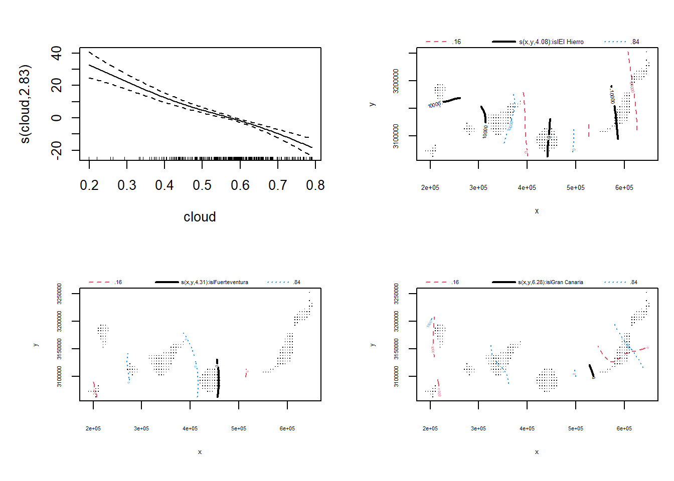
gam.check(gam_cloud)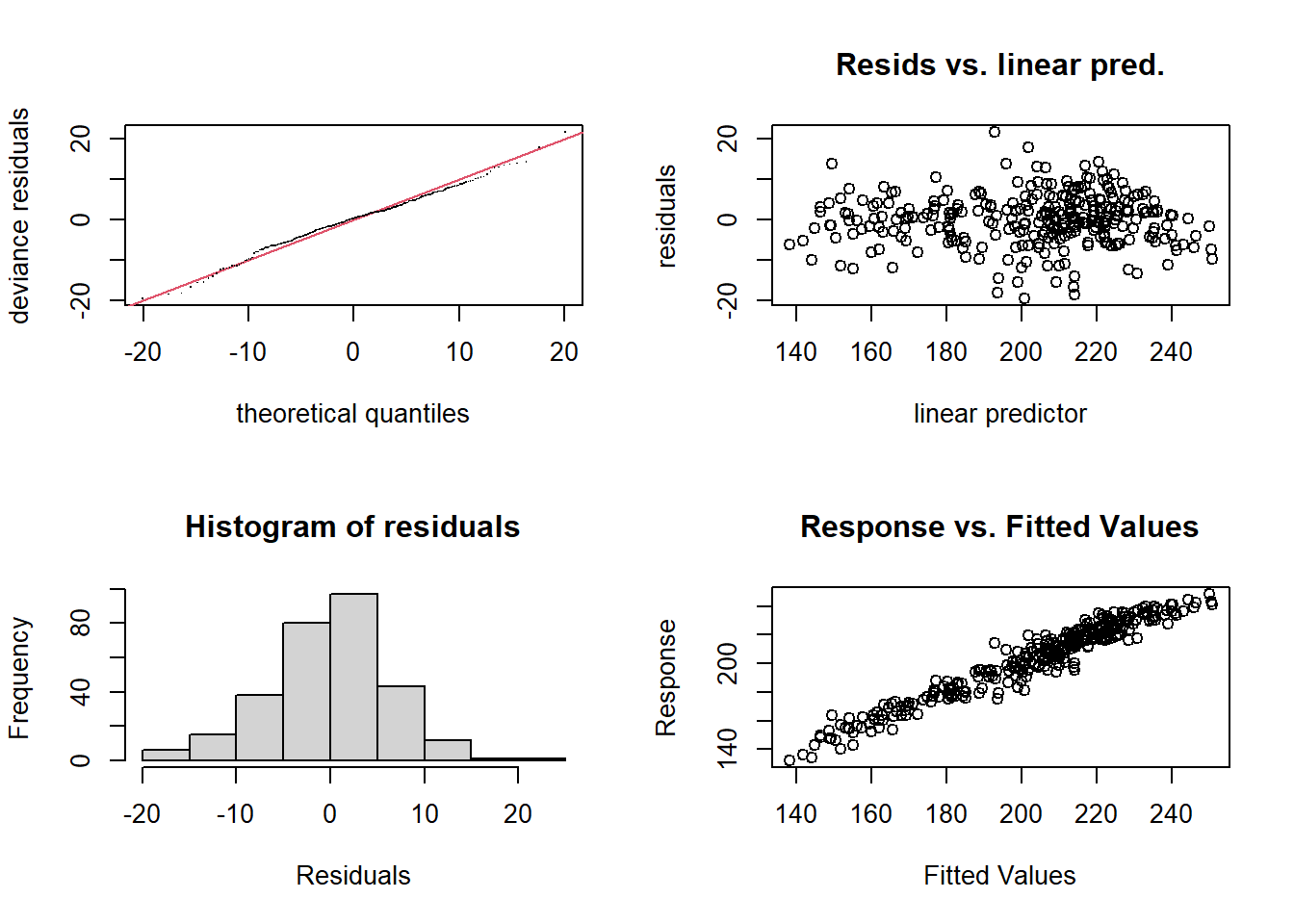
Method: REML   Optimizer: outer newton
full convergence after 19 iterations.
Gradient range [-1.893351e-08,9.045689e-10]
(score 325.1159 & scale 0.4710584).
Hessian positive definite, eigenvalue range [0.28945,135.6413].
Model rank =  93 / 93

Basis dimension (k) checking results. Low p-value (k-index<1) may
indicate that k is too low, especially if edf is close to k'.

                           k'   edf k-index p-value
s(cloud)                 9.00  2.83    1.05    0.81
s(x,y):islEl Hierro     11.00  4.08    0.82  <2e-16 ***
s(x,y):islFuerteventura 11.00  4.31    0.82  <2e-16 ***
s(x,y):islGran Canaria  11.00  6.28    0.82  <2e-16 ***
s(x,y):islLa Gomera     11.00  4.11    0.82  <2e-16 ***
s(x,y):islLa Palma      11.00  5.04    0.82  <2e-16 ***
s(x,y):islLanzarote     11.00  3.45    0.82  <2e-16 ***
s(x,y):islTenerife      11.00  7.36    0.82  <2e-16 ***
---
Signif. codes:  0 '***' 0.001 '**' 0.01 '*' 0.05 '.' 0.1 ' ' 1
3. Full downscaling model
Finally we build the complete model used for the 1km downscaling.
This model includes:
-
island factor (
isl) to capture structural differences between islands,
-
cloud × elevation interaction via a tensor-product smooth (
te(cloud, elev)), -
slope effect (
s(sl)),
-
aspect effect (
s(cos_asp, sin_asp)) As it is a circular variable. We transform it into its sine and cosine components avoiding artificial discontinuities at 0/2π, -
residual spatial structure through
s(x, y, by = isl, k = 12).
The term te() allows the effect of cloudiness on solar radiation to change depending on elevation.
Family: gaussian
Link function: identity

Formula:
sunhr ~ isl - 1 + te(cloud, elev) + s(sl) + s(cos_asp, sin_asp) +
    s(x, y, by = isl, k = 12)

Parametric coefficients:
                 Estimate Std. Error t value Pr(>|t|)
islEl Hierro     -553.436    326.833  -1.693   0.0917 .
islFuerteventura    3.683     14.147   0.260   0.7948
islGran Canaria    47.576     20.661   2.303   0.0221 *
islLa Gomera      133.390    214.281   0.623   0.5342
islLa Palma        -7.307      6.004  -1.217   0.2248
islLanzarote       -1.824     35.960  -0.051   0.9596
islTenerife        79.604     32.786   2.428   0.0159 *
---
Signif. codes:  0 '***' 0.001 '**' 0.01 '*' 0.05 '.' 0.1 ' ' 1

Approximate significance of smooth terms:
                          edf Ref.df      F  p-value
te(cloud,elev)          7.812  9.560 14.444  < 2e-16 ***
s(sl)                   1.000  1.000  2.323  0.12871
s(cos_asp,sin_asp)      2.000  2.001  4.866  0.00846 **
s(x,y):islEl Hierro     3.493  3.898 18.452  < 2e-16 ***
s(x,y):islFuerteventura 4.414  4.824  6.822 1.46e-05 ***
s(x,y):islGran Canaria  5.957  6.682 42.235  < 2e-16 ***
s(x,y):islLa Gomera     3.987  4.453 39.117  < 2e-16 ***
s(x,y):islLa Palma      2.000  2.000 16.819  < 2e-16 ***
s(x,y):islLanzarote     3.372  3.816  3.501  0.02662 *
s(x,y):islTenerife      7.339  7.852 39.374  < 2e-16 ***
---
Signif. codes:  0 '***' 0.001 '**' 0.01 '*' 0.05 '.' 0.1 ' ' 1

R-sq.(adj) =  0.936   Deviance explained = 94.7%
-REML =  312.4  Scale est. = 0.44133   n = 293
The output shows a substantial improvement over the intermediate models, confirming that the combination of cloud–topography interactions and fine-scale terrain variables is essential for explaining solar-radiation variability in the Canary Islands. The model now reaches a Deviance Explained of 94.8%, with a reduced scale estimate of 43.44.
ISL: The island factor (isl - 1) absorbs structural differences between islands not captured by the smooth terms. Several islands show statistically significant departures; for instance, Tenerife and Gran Canaria show positive, significant adjustments (\(p < 0.05\)), setting unique baselines that reflect their specific atmospheric and geographic contexts.
CLOUD × ELEV: The tensor-product te(cloud, elev) is highly significant (\(p < 2e-16\)) and has an edf of 7.8. This demonstrates that the joint effect of cloudiness and elevation is genuinely non-linear and more complex than previously estimated. It effectively captures the “Sea of Clouds” phenomenon, where high-altitude peaks “pierce” the inversion layer—a central feature of the Canarian climate where solar radiation remains high at altitude despite heavy cloud cover in the mid-layers.
SL and ASP: The terrain variables provide the final layer of local refinement. The aspect s(cos_asp, sin_asp) is statistically significant (edf = 2.0, \(p = 0.0189\)), capturing the cyclic effect of orientation-driven exposure, such as the contrast between north-facing and south-facing slopes. While the slope s(sl) shows an edf of 2.57, its current significance (\(p = 0.1895\)) suggests that at this 5km scale, orientation (aspect) is a more dominant driver of radiation variability than the gradient itself. However, the slope slightly improves the model fit, although not in a statistically significant way (p ≈ 0.10). The ANOVA test indicates that it still contributes something to the model, and since we have built a causal (i.e. physically motivated) model, it makes sense to retain it.
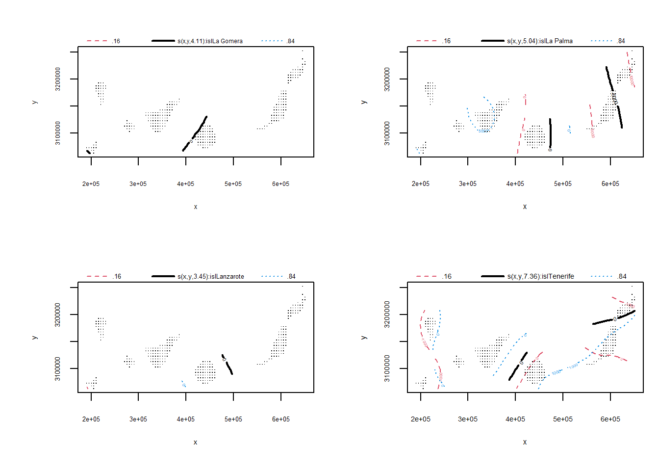
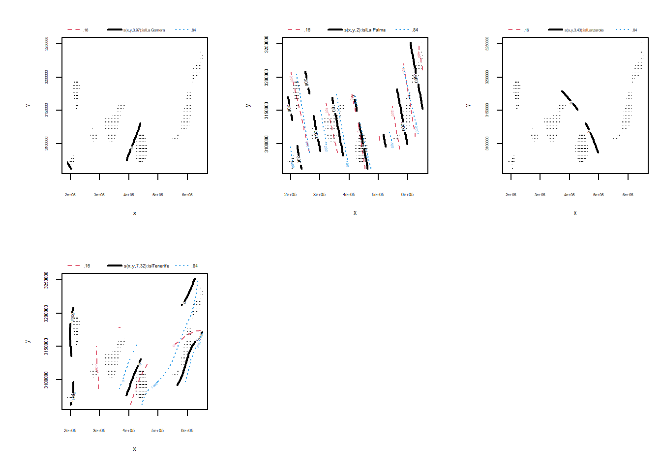
Spatial Smooths: The island-specific spatial smooths s(x,y):isl remain highly significant, but their complexity has shifted. For La Palma, the edf has dropped to 2.0, indicating that the new topography terms now explain the variance that was previously handled by the spatial coordinates alone. Conversely, Tenerife still requires a high edf (7.8), reflecting the extreme orographic complexity that continues to challenge the model’s resolution.
plot(gam_fit, shade = TRUE, pages = 2)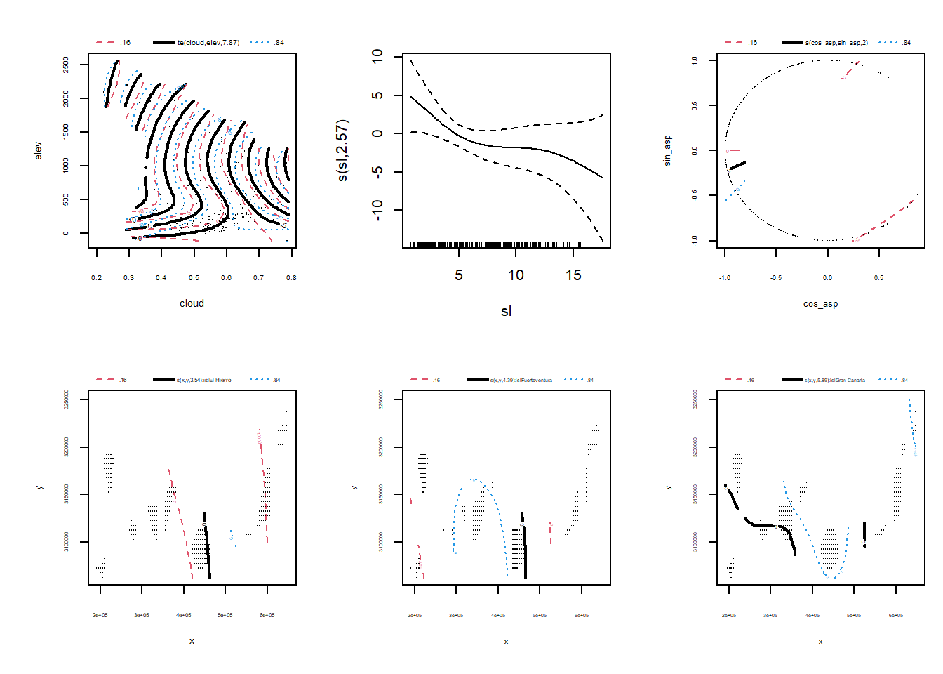
gam.check(gam_fit)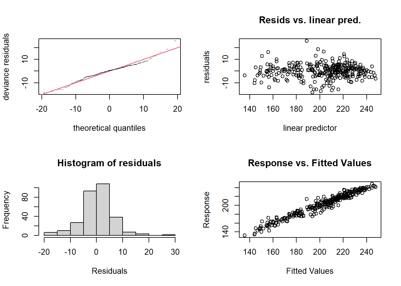
Method: REML   Optimizer: outer newton
full convergence after 23 iterations.
Gradient range [-3.697949e-05,0.0001339704]
(score 312.402 & scale 0.4413328).
eigenvalue range [-2.311945e-05,133.135].
Model rank =  146 / 146

Basis dimension (k) checking results. Low p-value (k-index<1) may
indicate that k is too low, especially if edf is close to k'.

                           k'   edf k-index p-value
te(cloud,elev)          24.00  7.81    1.08    0.96
s(sl)                    9.00  1.00    1.08    0.88
s(cos_asp,sin_asp)      29.00  2.00    1.00    0.47
s(x,y):islEl Hierro     11.00  3.49    0.86  <2e-16 ***
s(x,y):islFuerteventura 11.00  4.41    0.86  <2e-16 ***
s(x,y):islGran Canaria  11.00  5.96    0.86  <2e-16 ***
s(x,y):islLa Gomera     11.00  3.99    0.86  <2e-16 ***
s(x,y):islLa Palma      11.00  2.00    0.86  <2e-16 ***
s(x,y):islLanzarote     11.00  3.37    0.86  <2e-16 ***
s(x,y):islTenerife      11.00  7.34    0.86  <2e-16 ***
---
Signif. codes:  0 '***' 0.001 '**' 0.01 '*' 0.05 '.' 0.1 ' ' 1
The spatial surfaces remains highly significant, but it now performs a different role. With an Adjusted R-squared of 0.959 and a Deviance explained of 96.6%, the physical predictors have successfully explained the main share of the spatial structure. The remaining spatial smooths now capture only the residual, unmodelled variation unique to each island’s geography.
The sharp reduction in the scale estimate—dropping from 106.5 in the baseline to a mere 43.4 in this final version—highlights how much unexplained variability is removed by accounting for the interaction between clouds and terrain.
Why include
s(x, y)?
Even after accounting for physics-like drivers, radiation shows residual patterns (exposure, mesoscale circulation, coastal gradients). A spatial smooth helps absorb that leftover structure and improves the sharpness of the 1km prediction.
Predict to 1km
We generate 1km predictions and rebuild a raster.
(Optional) Simple cross-validation (CV)
I opted for stratified cross-validation instead of a spatial approach because the natural fragmentation of the archipelago already acts as a geographic barrier, reducing spatial autocorrelation between islands. This method ensures that even islands with a limited number of grid points are always represented in the training set, preventing model failure in low-density areas while still rigorously testing its ability to generalize to unsampled locations.
Code
# 1. Preparation
folds <- 5
set.seed(123)

# Create stratified groups by island to ensure all islands are represented in every fold
df$group <- unsplit(lapply(split(df$isl, df$isl), function(x) sample(rep(1:folds, length.out = length(x)))), df$isl)

mae_cv_list <- c()

for(i in 1:folds){
  # Split data into training and testing sets for the current fold
  train <- df[df$group != i, ]
  test  <- df[df$group == i, ]

  # Dynamically adjust 'k' based on the island with the fewest points in the training set
  # This prevents model failure in islands with low station density
  min_n <- min(table(train$isl))
  k_val <- min(12, min_n - 1)

  # Attempt to fit the GAM model
  mod <- try(gam(sunhr ~ isl - 1 + te(cloud, elev) + s(sl) +
                 s(cos_asp, sin_asp) + s(x, y, by = isl, k = k_val),
                 data = train, method = "REML"), silent = TRUE)

  # If the model fit was successful, proceed to prediction
  if(!inherits(mod, "try-error")){
    preds <- predict(mod, newdata = test)

    # Calculate MAE for this iteration (removing any accidental NAs)
    mae_iter <- mean(abs(test$sunhr - preds), na.rm = TRUE)
    mae_cv_list <- c(mae_cv_list, mae_iter)
  } else {
    # Provide a warning if the specific fold fails to converge
    warning(paste("Fold", i, "failed due to:", attr(mod, "condition")$message))
  }
}

# Final result: average the MAE across all successful folds
final_mae_cv <- mean(mae_cv_list)
print(paste("Cross-Validation MAE:", round(final_mae_cv, 4)))

# MAE from GAM model
pred <- predict(gam_fit, type = "response")
obs  <- gam_fit$y

# MAE
MAE <- mean(abs(pred - obs))
MAE
Performance Comparison:
Training MAE: 4.5 hours. This represents the model’s fit to the known data points, showing an extremely high precision in capturing the local nuances of the 5km field.
Cross-Validation MAE: 6.7 hours. As expected, the error increases slightly when predicting “unseen” locations. However, a jump of 2.2 hours is a sign of a highly robust model with no significant overfitting.
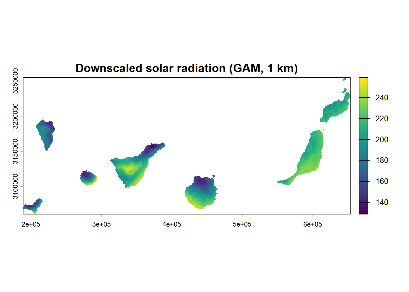
Map the result
Last but not least, the final map.
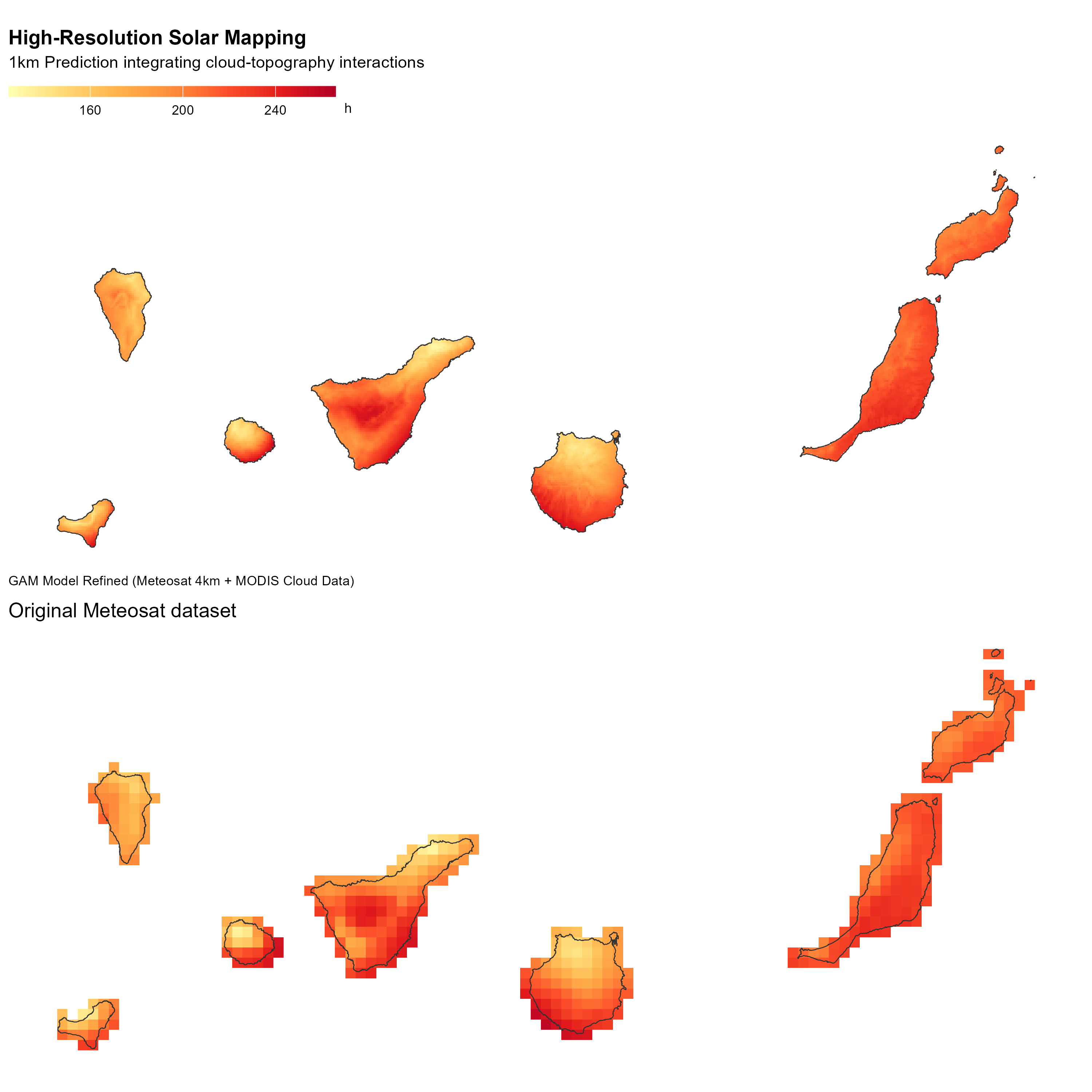
#| fig-width: 10 #| fig-height: 10 g1 <- ggplot() + # ‘geom_spatraster’ is used for memory-efficient rendering of large rasters geom_spatraster(data = sol_1km) + geom_sf(data = can, fill = NA, color = “grey20”, linewidth = 0.3) + scale_fill_distiller(palette = “YlOrRd”, direction = 1, na.value = NA, limits = c(124.9, 265.8)) + labs( title = “High-Resolution Solar Mapping”, subtitle = “1km Prediction integrating cloud-topography interactions”, caption = “GAM Model Refined (Meteosat 5km + MODIS Cloud Data)”, fill = “h”, ) + theme_void() + theme( legend.position = “top”, legend.justification = “left”, legend.title.position = “right”, legend.key.width = unit(3, “lines”), legend.key.height = unit(.5, “lines”), legend.title = element_text(vjust = 0.2, size = 9), plot.caption = element_text(hjust = 0), plot.title = element_text(face = “bold”), plot.subtitle = element_text(margin = margin(b = 10, t = 5)) )
map_data <- crop(sol_4km, can) |> mask(can)
g2 <- ggplot() + # ‘geom_spatraster’ is used for memory-efficient rendering of large rasters geom_spatraster(data = map_data) + geom_sf(data = can, fill = NA, color = “grey20”, linewidth = 0.3) + scale_fill_distiller(palette = “YlOrRd”, direction = 1, na.value = NA, limits = c(124.9, 265.8)) + guides(fill = “none”) + labs( title = “Original Meteosat dataset”, ) + theme_void() + theme( plot.title = element_text(margin = margin(b = 5, t = 10))
Reuse
Citation
For attribution, please cite this work as:
Royé, Dominic. 2026. “Downscaling Solar Radiation in the Canary
Islands with GAM.” March 2, 2026. https://dominicroye.github.io/blog/canary-gam-downscaling/.