Map projections: a practical guide to common mistakes and how to fix them
R
R:Intermediate
Visualization
Maps
Bad practice
Projections
GIS
Author
Dominic Royé
Published
May 3, 2026
If you have spent any time reading scientific journals, news outlets, or even peer-reviewed climate research, you have almost certainly encountered a world map stretched beyond recognition, with continents bloated at the poles, Greenland looming as large as Africa, or a country’s area visually misrepresented because of an inappropriate coordinate reference system. Map projections are one of the most systematically overlooked aspects of cartographic communication, and the consequences go beyond aesthetics: a wrong projection can actively mislead the reader, distort spatial relationships, and undermine the scientific message.
In this post I want to offer a practical guide, grounded in both cartographic theory and real R code, to help you choose the right projection for your purpose and avoid the most common pitfalls.
Why projections matter
The Earth is (approximately) a sphere. A map is flat. Translating a curved surface onto a plane inevitably introduces distortion, and no projection can simultaneously preserve all of the following properties:
Area relative sizes of regions are maintained (equal-area or equivalent projections)
Shape local angles are preserved, so small regions look correct (conformal projections)
Distance distances from one or two specific points are preserved (equidistant projections)
Direction bearings from a central point are preserved (azimuthal projections)
Every projection is a compromise, trading distortion of one property for accuracy in another. The critical question is therefore not “which projection is best?” but rather “which distortion is acceptable for my specific purpose?”
TipThe key rule
Match the projection to the purpose. A projection used for navigation is not appropriate for a choropleth showing disease incidence. A projection ideal for a continental map of Europe is not suitable for a global map of biodiversity.
Packages
Package
Description
tidyverse
Collection of packages (visualization, manipulation): ggplot2, dplyr, purrr, etc.
sf
Simple Feature: import, export and manipulate vector data
terra
Import, export, manipulate and project raster (and vector) data
giscoR
Eurostat GISCO API: administrative boundaries for Europe and the world
patchwork
Compose multiple ggplot2 plots into a single figure
ggtext
Improved text rendering for ggplot2 (HTML/Markdown in labels)
The offenders: projections you should stop using (for most things)
Mercator | the world’s most misused projection
The Mercator projection was designed in 1569 by Gerardus Mercator for nautical navigation. It is a conformal projection, meaning it preserves local angles and shapes perfectly, which is exactly what sailors needed to plot straight compass bearings. For that specific purpose, it remains excellent.
The problem is that Mercator dramatically exaggerates areas away from the equator. At 60° latitude, areas appear roughly four times larger than they actually are. Greenland is the most striking example: it looks comparable in size to Africa, when in reality Africa is about 14 times larger. Yet Mercator is still routinely used in scientific publications for choropleth maps, and global thematic analyses.
When is Mercator acceptable?
Web map tiles and interactive maps (OpenStreetMap), its conformal properties make tile seams invisible and it remains the de facto standard for tiled web maps at street to country scale
Large-scale navigation charts
Conformal mapping of small areas where distortion is negligible
NoteGoogle moved away from Mercator at global scale
In August 2018, Google Maps switched to a 3D globe view when zoomed out to world scale, replacing the flat Mercator canvas it had used since launch. The stated reason was exactly the distortion problem described here.
When should you never use Mercator?
Any thematic map where area size conveys information (choropleth, dot density, proportional symbols)
Global or hemispheric maps
Maps communicating spatial patterns of phenomena with area-dependent interpretations (e.g., biodiversity, population density, climate zones)
Code
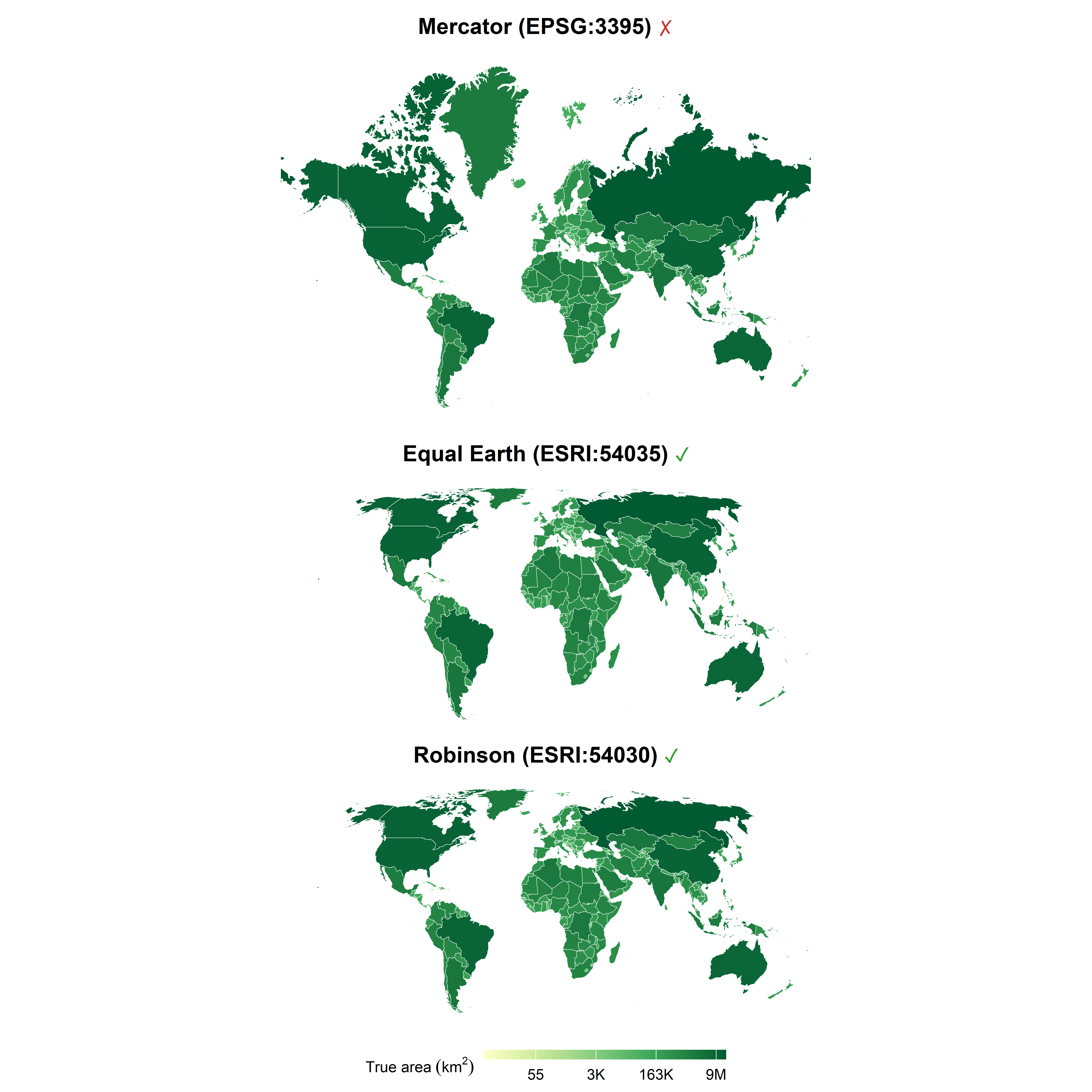
# world countries from giscoR (low resolution, geographic CRS)world<-gisco_get_countries(year ="2020", resolution ="10", epsg ="4326")|>filter(CNTR_ID!="AQ")|># remove Antarcticast_make_valid()# repair any degenerate geometries# compute land area (km^2): because sf_use_s2(FALSE) forces planar geometry,# we must project to an equal-area CRS first so that st_area() gives# correct results (planar area on an equal-area projection = true geodesic area)world<-world|>mutate(area_km2 =as.numeric(st_area(st_transform(geometry, "ESRI:54035")))/1e6)# colour \u2713 green and \u2717 red using HTML spans (rendered via element_markdown)color_sym<-function(x){x<-gsub("\u2713", "<span style='color:#2a9e2a'>✓</span>", x, fixed =TRUE)x<-gsub("\u2717", "<span style='color:#cc3333'>✗</span>", x, fixed =TRUE)x}# helper: build one map panelmake_map<-function(data, crs_string, title){data_proj<-st_transform(data, crs_string)ggplot(data_proj)+geom_sf(aes(fill =area_km2), color ="white", linewidth =0.15)+coord_sf(default_crs =NULL)+scale_fill_distiller( palette ="YlGn", direction =1, name =expression("True area"~(km^2)), trans ="log", labels =~scales::number(., accuracy =1, scale_cut =scales::cut_short_scale()))+labs(title =color_sym(title))+theme_void(base_size =11)+theme( plot.title =element_markdown(face ="bold", hjust =0.5, margin =margin(b =6, t =5)), legend.position ="bottom", legend.key.width =unit(2, "lines"), legend.title =element_text(size =9), legend.key.height =unit(.4, "lines"),)}p_mercator<-make_map(world, "EPSG:3395", "Mercator (EPSG:3395) \u2717")p_eqearth<-make_map(world, "ESRI:54035", "Equal Earth (ESRI:54035) \u2713")p_robinson<-make_map(world, "ESRI:54030", "Robinson (ESRI:54030) \u2713")((p_mercator/p_eqearth/p_robinson)+plot_layout(guides ="collect"))&theme(legend.position ="bottom")
The visual difference is striking. Even when the fill colour encodes the true area (computed in an equal-area projection), the Mercator panel makes Canada, Russia, and Greenland dominate the canvas, even though Mercator inflates them beyond their already large actual area, creating a systematic visual bias. In Equal Earth and Robinson, the polygon size and the fill colour tell the same story.
Geographic coordinates
Almost as common as Mercator, and almost as problematic for thematic maps, is simply plotting data in geographic (longitude/latitude) coordinates, i.e., treating degrees as Cartesian x/y coordinates. This is sometimes called the equirectangular projection (EPSG:4326 used as a projection rather than a geographic CRS). It is not conformal, not equal-area, and not equidistant in a meaningful global sense. It is, however, the default when you load spatial data and forget to set a projection. In R, if you pass an sf object to ggplot2 without specifying coord_sf(crs = ...), you are implicitly using this projection.
WarningWatch your defaults in ggplot2
When you call geom_sf() without explicitly setting coord_sf(crs = ...), ggplot2 uses the native CRS of the data, usually WGS84 (EPSG:4326). While this is fine for inspection, it is not appropriate for final publication maps covering large areas.
A taxonomy of projections by purpose
Before looking at specific recommendations, it helps to understand the main families:
Family
Property preserved
Typical use
Equal-area (equivalent)
Area
Choropleth, density, species richness, climate zones
Conformal
Local shape/angles
Navigation, large-scale topographic maps
Compromise
Neither fully, but balanced distortion
General-purpose reference maps, atlases
Azimuthal
Direction from center
Polar maps, great-circle routes
Equidistant
Distance from one or two points
Maps centered on a specific location
Practical recommendations by context
Global thematic maps: use equal-area projections
For any global map where the visual weight of a region should reflect its actual area, an equal-area projection is mandatory. The main options are:
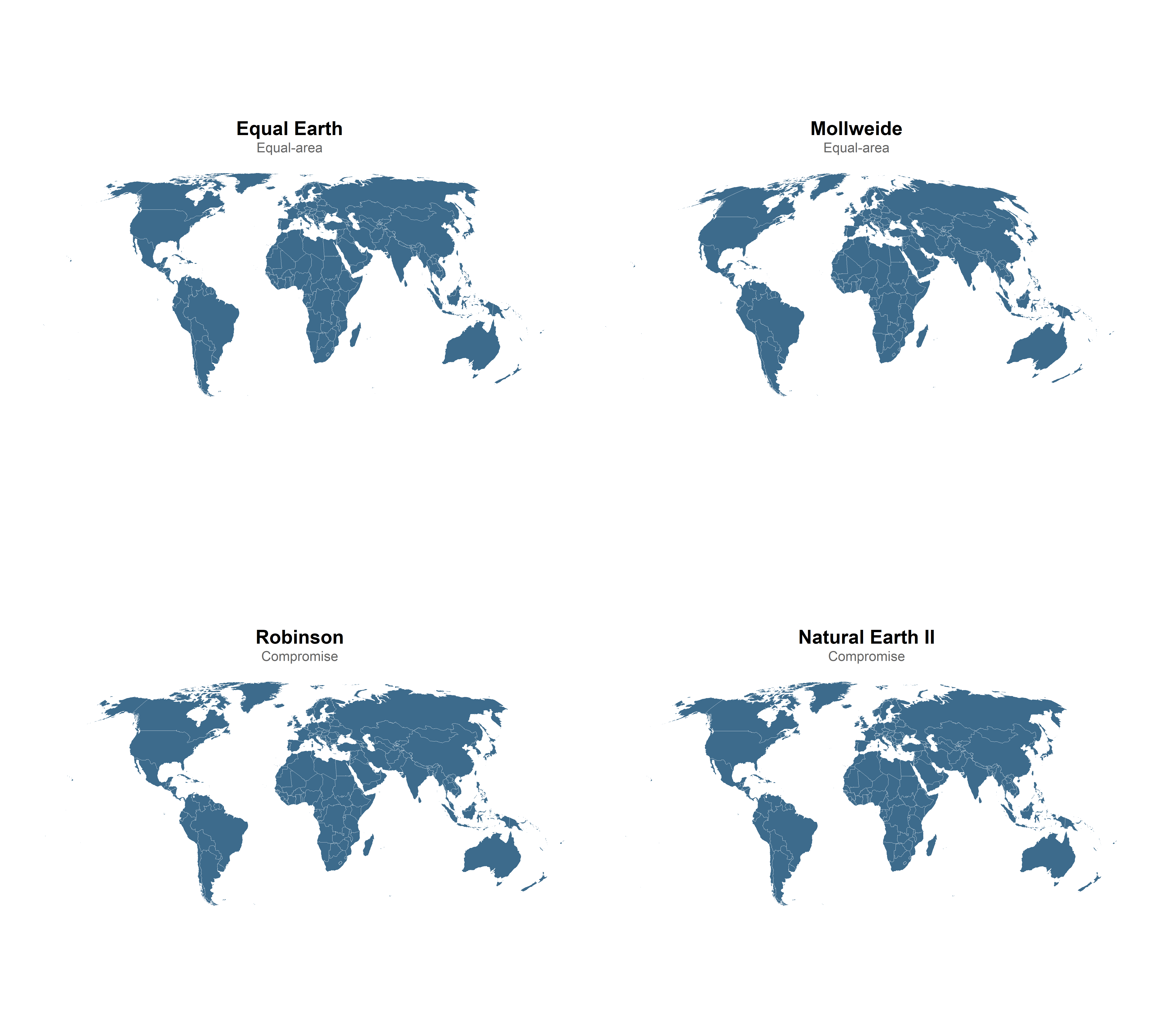
Equal Earth (ESRI:54035): A pseudocylindrical equal-area projection designed in 2018, specifically created as a modern replacement for Robinson. It has a pleasing appearance and correctly represents relative areas. This is currently the recommended choice for world thematic maps.
Mollweide (ESRI:54009): Classic pseudocylindrical equal-area projection, widely used in scientific journals. Shapes are distorted toward the edges but areas are perfectly preserved. A solid choice.
Goode’s Homolosine (ESRI:54052): Interrupts the ocean to reduce continental distortion. Useful when land areas are the focus and visual interruptions in the ocean are acceptable.
Robinson (ESRI:54030): A compromise projection: it is not equal-area, but the area distortions are modest and it has a visually balanced appearance. Widely used by National Geographic and the USGS for general-purpose world maps. Acceptable for reference maps but not for thematic maps where area comparison matters.
Natural Earth II (ESRI:54078): A compromise projection designed by Tom Patterson (US National Park Service) with a pleasing rounded appearance at the poles. A practical and widely used alternative to Winkel Tripel for general-purpose world maps. Note that Winkel Tripel (ESRI:54042) is another popular choice, but it can cause geometry exceptions in certain software configurations, so Natural Earth II (ESRI:54078) is the safer option in R.
How to visually verify area distortion: the Tissot indicatrix
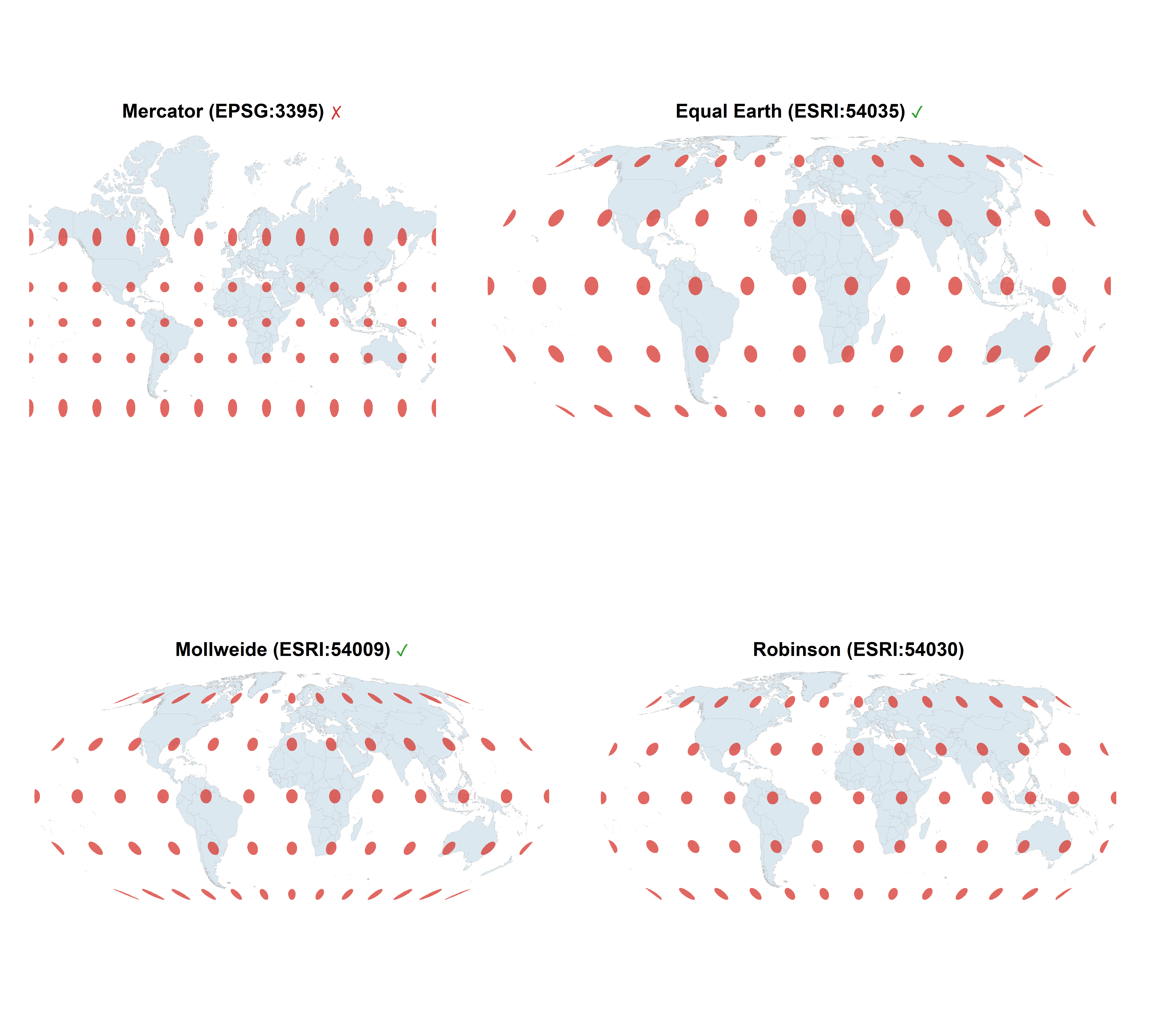
A classic tool for visualizing projection distortion is Tissot’s indicatrix, a set of circles of identical size placed at regular intervals across the globe in the unprojected space. If the projection preserves area, all circles will have the same area on the map (though their shapes may differ). If the projection is conformal, all circles will remain circular (though sizes may differ).
Code
# generate Tissot indicatrix circles in WGS84generate_tissot<-function(spacing=30, radius_deg=4){lons<-seq(-180, 180, by =spacing)lats<-seq(-60, 60, by =spacing)grid<-expand.grid(lon =lons, lat =lats)circles<-pmap(grid, function(lon, lat){# approximate circle in geographic spaceangles<-c(seq(0, 2*pi, length.out =64), 0)xs<-lon+radius_deg*cos(angles)ys<-lat+radius_deg*sin(angles)# clampxs<-pmax(-179.9, pmin(179.9, xs))ys<-pmax(-89.9, pmin(89.9, ys))st_polygon(list(cbind(xs, ys)))})st_sf(geometry =st_sfc(circles, crs =4326))}tissot<-generate_tissot()graticule<-st_graticule(ndiscr =10000, margin =0.001)make_tissot_map<-function(world, tissot, crs_string, title){world_proj<-st_transform(world, crs_string)tissot_proj<-st_transform(tissot, crs_string)ggplot()+geom_sf(data =world_proj, fill ="#dce8f0", color ="grey70", linewidth =0.1)+geom_sf(data =tissot_proj, fill ="#d7362d", color =NA, alpha =0.75)+coord_sf(default_crs =NULL)+labs(title =color_sym(title))+theme_void(base_size =10)+theme(plot.title =element_markdown(face ="bold", hjust =0.5))}t1<-make_tissot_map(world, tissot, "EPSG:3395", "Mercator (EPSG:3395) \u2717")t2<-make_tissot_map(world, tissot, "ESRI:54035", "Equal Earth (ESRI:54035) \u2713")t3<-make_tissot_map(world, tissot, "ESRI:54009", "Mollweide (ESRI:54009) \u2713")t4<-make_tissot_map(world, tissot, "ESRI:54030", "Robinson (ESRI:54030)")(t1|t2)/(t3|t4)
The Mercator indicatrix makes the distortion at high latitudes unmistakable. On the equal-area projections, every red circle has the same area, which is exactly what we want for any thematic map.
Regional and continental maps
For maps of continents or large sub-continental regions, the choice of projection depends on the shape of the region (east-west vs. north-south extent) and, again, the purpose.
Europe: The standard for European statistical maps, used by Eurostat, the EU, and most national mapping agencies, is the Lambert Azimuthal Equal Area (LAEA) centered on Europe, EPSG:3035. It is the projection you should use for any choropleth or spatial analysis of European data.
North America (continental USA): The Albers Equal Area Conic (EPSG:5070 or ESRI:102003) is the standard. It minimizes distortion across the broad east-west extent of the USA.
Spain / Iberian Peninsula: For maps of Spain or the Iberian Peninsula, the UTM zone 30N (EPSG:25830) is appropriate for large-scale work. For smaller scale or country-level maps a LCC or LAEA centered on Spain also works well.
Polar regions: Use an azimuthal equal-area (e.g., NSIDC Sea Ice Polar Stereographic, EPSG:3413 for the Arctic, EPSG:3976 for Antarctic) or a polar stereographic projection.
Code
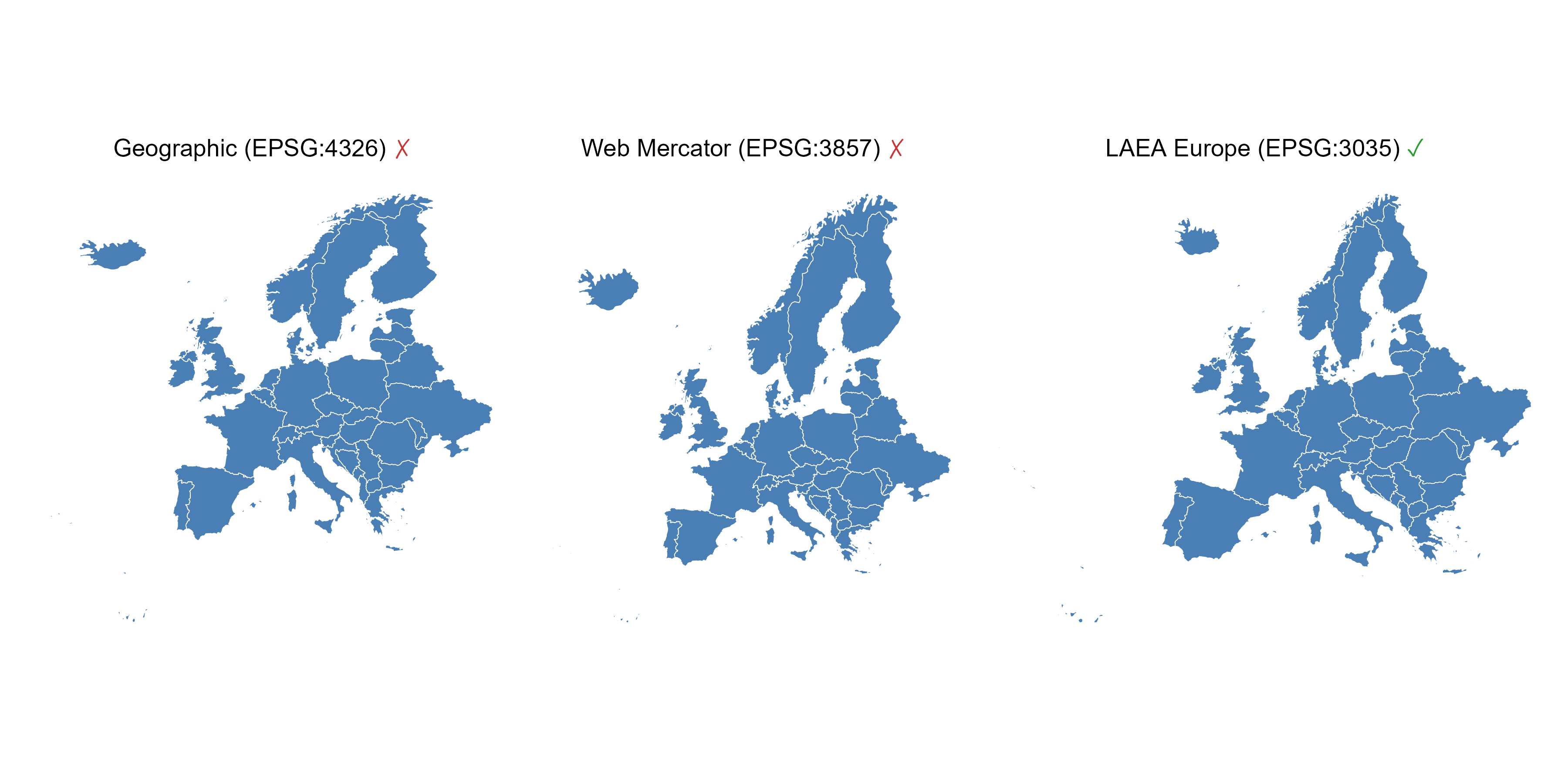
# European countries from giscoReurope<-gisco_get_countries( region ="Europe", resolution ="10", year ="2020")|>filter(!CNTR_ID%in%c("GL", "SJ", "RU"))|># remove Greenland, Svalbard, Russiast_crop(xmin =-33, xmax =50, ymin =26, ymax =75)# remove French Guianamake_europe_map<-function(data, crs_string, title){data_proj<-st_transform(data, crs_string)ggplot(data_proj)+geom_sf(fill ="#4a7fb5", color ="white", linewidth =0.2)+coord_sf(default_crs =NULL, expand =TRUE)+labs(title =color_sym(title))+theme_void(base_size =11)+theme( plot.title =element_markdown(hjust =0.5, margin =margin(b =6)))}e1<-make_europe_map(europe, 4326, "Geographic (EPSG:4326) \u2717")e2<-make_europe_map(europe, 3857, "Web Mercator (EPSG:3857) \u2717")e3<-make_europe_map(europe, 3035, "LAEA Europe (EPSG:3035) \u2713")e1|e2|e3
The difference between Web Mercator and LAEA is particularly visible: Scandinavia appears oversized and the overall shape of Europe looks squashed under Mercator, while LAEA gives the correct, familiar shape that European institutions use.
Hemispheric and “globe-view” maps: the Orthographic projection
The Orthographic projection (+proj=ortho) renders the Earth as if viewed from space, giving a hemisphere perspective that is visually compelling and immediately intuitive for a general audience. The compression toward the edges of the visible hemisphere is not a cartographic flaw in the traditional sense: it is an accurate consequence of perspective geometry, the same foreshortening you see in a photograph of a sphere. Because readers instinctively interpret it as a three-dimensional object, the compression is cognitively transparent in a way that Mercator’s area inflation is not. That said, orthographic is not suitable for any analysis where areas or distances are measured from the map directly, so use an equal-area or equidistant projection for that. The center of the visible hemisphere is controlled by +lat_0 (latitude) and +lon_0 (longitude). For a Europe-centered view:
WarningGeometries must be clipped to the visible hemisphere before projecting
This is the main difficulty with the Orthographic projection. Any geometry that crosses the horizon (the boundary between the visible and hidden hemisphere) will produce incorrect or broken shapes after projection, because sf will attempt to project coordinates that are mathematically behind the globe, yielding nonsensical results.
The standard solution is to intersect all vector data with a circle of Earth’s radius centred at the projection origin, in the orthographic CRS, before transforming:
ortho_crs<-'+proj=ortho +lat_0=51 +lon_0=0.5 +x_0=0 +y_0=0 +R=6371000 +units=m +no_defs +type=crs'# 1. Build the visible hemisphere boundary (circle of Earth radius at origin)hemisphere<-st_point(c(0, 0))|>st_sfc(crs =ortho_crs)|>st_buffer(dist =6371000)# Earth radius in metres# 2. Transform world to orthographic, then clip to the visible hemisphereworld_ortho<-world|>st_transform(crs =ortho_crs)|>st_intersection(hemisphere)# 3. Same for graticulesgraticule_ortho<-st_graticule(ndiscr =10000, margin =0.001)|>st_transform(crs =ortho_crs)|>st_intersection(hemisphere)# 4. The hemisphere circle also serves as the ocean/globe backgroundggplot()+geom_sf(data =hemisphere, fill ="#cce4f0", color =NA)+# oceangeom_sf(data =world_ortho, fill ="#3d6b8c", color ="white", linewidth =0.1)+geom_sf(data =graticule_ortho, color ="white", linewidth =0.1, alpha =0.5)+coord_sf(crs =ortho_crs)+theme_void()
For raster data in orthographic projection, terra::project() handles the reprojection cleanly, but you should convert to a data.frame afterwards and use geom_raster() rather than geom_spatraster():
Specifying projections in R with sf, ggplot2, and terra
In practice, working with projections in R is straightforward. Below are the most common patterns for both vector data (sf) and raster data (terra).
Vector data with sf and ggplot2
# 1. Inspect the CRS of an sf objectst_crs(my_sf)# full CRS object (prints WKT2)st_crs(my_sf)$epsg# EPSG code as integer (NA if none)st_crs(my_sf)$Name# human-readable namest_crs(my_sf)$wkt# WKT2 string - the authoritative representation# 2. Transform to a different CRSmy_sf_laea<-st_transform(my_sf, "EPSG:3035")# EPSG code - preferred as code or stringmy_sf_ee<-st_transform(my_sf, "ESRI:54035")# ESRI code - preferred for world projectionsmy_sf_laea<-st_transform(my_sf, st_crs(my_sf)$wkt)# WKT2 string - portable/archival# 3. Set projection for display only in ggplot2 (data are not transformed)ggplot(my_sf)+geom_sf()+coord_sf(crs =3035)# LAEA Europeggplot(my_sf)+geom_sf()+coord_sf(crs ="ESRI:54035")# Equal Earthggplot(my_sf)+geom_sf()+coord_sf(crs ="ESRI:54009")# Mollweideggplot(my_sf)+geom_sf()+coord_sf(crs ="ESRI:54030")# Robinson# 4. Obtain the WKT2 of any CRS from its EPSG code (useful for sharing/archiving)wkt_laea<-st_crs("EPSG:3035")$wktcat(wkt_laea)
Raster data with terra
Projecting rasters requires resampling, every output cell must be filled by interpolating from the input grid. The choice of resampling method matters: use "bilinear" (or "cubic") for continuous variables like temperature or elevation, and "near" (nearest neighbour) for categorical data like land cover classes.
# 1. Inspect the CRS of a SpatRastercrs(my_raster)# returns a WKT2 stringcrs(my_raster, describe =TRUE)# compact human-readable summary# 2. Project using EPSG codes - preferred as string for standard CRSr_laea<-project(my_raster, "EPSG:3035")# LAEA Europer_aea_us<-project(my_raster, "EPSG:5070")# Albers Equal Area (USA)r_utm30<-project(my_raster, "EPSG:25830")# UTM zone 30N (Spain)# 3. Project using ESRI codes - preferred for world projections without EPSGr_eqearth<-project(my_raster, "ESRI:54035")# Equal Earthr_moll<-project(my_raster, "ESRI:54009")# Mollweider_robin<-project(my_raster, "ESRI:54030")# Robinson# 4. Project using a WKT2 string - the formal standard; use for archiving or# sharing CRS definitions, or when EPSG/ESRI codes are unavailablewkt_laea<-crs("EPSG:3035")# obtain WKT2 from an EPSG coder_laea<-project(my_raster, wkt_laea)# project using that WKT2# 5. Project to match an existing raster or vector objectr_matched<-project(my_raster, ref_raster)# match CRS, extent and resolutionr_matched<-project(my_raster, crs(my_sf))# match the CRS of an sf object# 6. Choose the resampling method explicitly (always do this consciously)r_temp<-project(my_raster, "EPSG:3035", method ="bilinear")# continuous datar_lc<-project(my_raster, "EPSG:3035", method ="near")# categorical data# 7. Align two rasters to an identical gridr_aligned<-project(my_raster, ref_raster, method ="bilinear")
Warningst_area(), s2, and projections know what your engine is doing
By default (sf > 1.0), st_area() uses the s2 spherical geometry engine, which computes geodesic area directly on WGS84 data no projection required and the result is correct:
If you have disabled s2 (sf_use_s2(FALSE)), the engine switches to planar GEOS geometry. In that case, st_area() on WGS84 data gives wrong results (it treats degrees as metres). You must project to an equal-area CRS first:
sf_use_s2(FALSE)st_area(my_sf_wgs84)# wrong: planar on degreesst_area(st_transform(my_sf_wgs84, "ESRI:54035"))# correct: planar on Equal Earth
For raster data, terra::expanse() always computes geodesic cell area regardless of projection the safest option when the CRS setting is uncertain.
TipHow to specify a CRS in R: EPSG, ESRI, WKT2, and legacy PROJ strings
There are several ways to identify a coordinate reference system in R. Knowing the difference matters.
EPSG codes ("EPSG:XXXX" or just the integer) come from the EPSG Geodetic Parameter Dataset, maintained by the IOGP. They cover most standard geodetic CRS used in national and international mapping. Examples: "EPSG:4326" (WGS84), "EPSG:3035" (LAEA Europe), "EPSG:3857" (Web Mercator).
ESRI codes ("ESRI:XXXXX") are identifiers from Esri’s projection engine, covering many world projections not registered in EPSG, such as Equal Earth (ESRI:54035), Robinson (ESRI:54030), and Mollweide (ESRI:54009). Both sf and terra resolve these codes via the PROJ library.
WKT2 (ISO 19162:2019) is the current formal standard for encoding CRS definitions as portable, human-readable text. It replaced the older WKT1 format and the legacy PROJ string format. Since PROJ 6 (2019), all major geospatial libraries, including sf, terra, GDAL, and QGIS, use WKT2 internally. When sharing or archiving CRS definitions, WKT2 is the recommended format.
Legacy PROJ strings (e.g., +proj=laea +lat_0=52 +lon_0=10 +ellps=GRS80) were the de facto standard before PROJ 6. They are still accepted by most software for backwards compatibility, but are deprecated: they can silently lose datum parameters compared to WKT2. Avoid them in new code.
# Obtain the WKT2 of any CRS and inspect itcat(st_crs("EPSG:3035")$wkt)# sfcat(crs("EPSG:3035"))# terra
ImportantRaster vs. vector: projection in ggplot2 is not the same
This is one of the most common sources of confusion when moving between vector and raster workflows.
Vector data (sf) can be projected on the fly inside coord_sf(). When you write:
ggplot2 reprojects the geometries during rendering. The underlying sf object is never modified; the transformation happens only for display. This is convenient for quick exploration.
Raster data (terra) does not support on-the-fly projection in ggplot2. Functions like geom_spatraster() (from the tidyterra package) draw the raster in its native CRS. If you need a different projection, you must explicitly call terra::project() before plotting:
# Wrong: the raster stays in its original CRS regardless of coord_sf(crs = ...)ggplot()+geom_spatraster(data =my_raster)+coord_sf(crs ="EPSG:3035")# has no effect on the raster# Correct: project the raster first, then plotmy_raster_proj<-project(my_raster, "EPSG:3035", method ="bilinear")ggplot()+geom_spatraster(data =my_raster_proj)+coord_sf(default_crs =NULL)
The default_crs parameter in coord_sf() controls how ggplot2 interprets the coordinate axes when computing plot limits. By default, ggplot2 assumes unprojected geographic data (WGS84, EPSG:4326), so it back-transforms axis limits to longitude/latitude before applying them. This works fine when data are in geographic coordinates, but causes errors or wrong extents when the data have already been projected to a Cartesian CRS (e.g., EPSG:3035 in metres).
Setting default_crs = NULL tells ggplot2 to treat the coordinates as plain Cartesian values and skip any back-transformation of axis limits. Use default_crs = NULL whenever your data are pre-projected:
# Data already in EPSG:3035 (metres) - use default_crs = NULLmy_sf_laea<-st_transform(my_sf, "EPSG:3035")ggplot(my_sf_laea)+geom_sf()+coord_sf(default_crs =NULL)# Equivalently, for rasters already projected:my_raster_proj<-project(my_raster, "EPSG:3035")ggplot()+geom_spatraster(data =my_raster_proj)+coord_sf(default_crs =NULL)
In summary:
Data type
On-the-fly projection via coord_sf(crs = ...)?
Pre-project before plotting?
Vector (sf)
Yes
Optional (recommended for complex CRS)
Raster (terra)
No
Always required
Quick-reference: projection codes for common use cases
Use case
Projection
Code
World thematic maps (choropleth, density)
Equal Earth
ESRI:54035
World thematic maps (alternative)
Mollweide
ESRI:54009
World reference/atlas maps
Robinson
ESRI:54030
World reference/atlas maps (alternative)
Natural Earth II
ESRI:54078
European thematic/statistical maps
LAEA Europe
EPSG:3035
USA thematic/statistical maps
Albers Equal Area (USA)
EPSG:5070
Iberian Peninsula / Spain
UTM zone 30N
EPSG:25830
Arctic maps
NSIDC Sea Ice Polar Stereographic N
EPSG:3413
Antarctic maps
NSIDC Sea Ice Polar Stereographic S
EPSG:3976
Web/tile maps (navigation, base layers)
Web Mercator
EPSG:3857
Navigation charts
Mercator
EPSG:3395
WGS84 geographic CRS (data storage/exchange)
-
EPSG:4326
Checklist: common projection mistakes in scientific publications
Before submitting a map to a journal or report, run through this checklist:
Does the map use Mercator for a thematic purpose? Mercator distorts area severely at high latitudes. Replace with an equal-area projection.
Are geographic coordinates (EPSG:4326) used as a projection? Treating degrees as Cartesian is technically the equirectangular projection, which is neither equal-area nor conformal. Reproject to a suitable CRS.
Is the projection appropriate for the region? A world projection applied to a continental map (or vice versa) introduces unnecessary distortion. Match the projection to the spatial extent.
For choropleth maps: is the projection equal-area? Area-dependent visualisations (choropleth, dot density, proportional symbols) require an equal-area projection. Conformal or compromise projections will mislead the reader.
For raster data: was the raster explicitly projected before analysis? Analysing or visualising raster data in an inappropriate CRS leads to incorrect spatial statistics. Always project explicitly with terra::project().
Is st_area() being called on WGS84 data with s2 disabled? If sf_use_s2(FALSE), area calculations on unprojected data are wrong. Project to an equal-area CRS first.