Accessing OpenStreetMap data with R
The database of Open Street Maps
Recently I created a map of the distribution of gas stations and electric charging stations in Europe.
Population density through the number of gas stations in Europe. #dataviz @AGE_Oficial @mipazos @simongerman600 @openstreetmap pic.twitter.com/eIUx2yn7ej
— Dr. Dominic Royé (@dr_xeo) February 25, 2018
How can you obtain this data?
Well, in this case I used points of interest (POIs) from the database of Open Street Maps (OSM). Obviously OSM not only contains streets and highways, but also information that can be useful when we use a map such as locations of hospitals or gas stations. To avoid downloading the entire OSM and extracting the required information, you can use an overpass API, which allows us to query the OSM database with our own criteria.
An easy way to access an overpass API is through overpass-turbo.eu, which even includes a wizard to build a query and display the results on a interactive map. A detailed explanation of the previous web can be found here. However, we have at our disposal a package osmdata that allows us to create and make queries directly from the R environment. Nevertheless, the use of the overpass-turbo.eu can be useful when we are not sure what we are looking for or when we have some difficulty in building the query.
Accessing the overpass API from R
The first step is to install several packages, in case they are not installed. In almost all my scripts I use tidyverse which is a fundamental collection of different packages, including dplyr (data manipulation), ggplot2 (visualization), etc. The sf package is the new standard for working with spatial data and is compatible with ggplot2 and dplyr. Finally, ggmap makes it easier for us to create maps.
#install the osmdata, sf, tidyverse and ggmap package
if(!require("osmdata")) install.packages("osmdata")
if(!require("tidyverse")) install.packages("tidyverse")
if(!require("sf")) install.packages("sf")
if(!require("ggmap")) install.packages("ggmap")

#load packages
library(tidyverse)
library(osmdata)
library(sf)
library(ggmap)
Build a query
Before creating a query, we need to know what we can filter. The available_features( ) function returns a list of available OSM features that have different tags. More details are available in the OSM wiki here.
For example, the feature shop contains several tags among others supermarket, fishing, books, etc.
#the first five features
head(available_features())
## [1] "4wd_only" "abandoned" "abutters" "access" "addr" "addr:city"#amenities
head(available_tags("amenity"))## [1] "animal_boarding" "animal_breeding" "animal_shelter" "arts_centre"
## [5] "atm" "baby_hatch"#shops
head(available_tags("shop"))## [1] "agrarian" "alcohol" "anime" "antiques" "appliance" "art"The first query: Where are cinemas in Madrid?
To build the query, we use the pipe operator %>%, which helps to chain several functions without assigning the result to a new object. Its use is very extended especially within the tidyverse package collection. If you want to know more about its use, you can find here a tutorial.
In the first part of the query we need to indicate the place where we want to extract the information. The getbb( ) function creates a boundering box for a given place, looking for the name. The main function is opq( ) which build the final query. We add our filter criteria with the add_osm_feature( ) function. In this first query we will look for cinemas in Madrid. That’s why we use as key amenity and cinema as tag. There are several formats to obtain the resulting spatial data of the query. The osmdata_*( ) function sends the query to the server and, depending on the suffix * sf/sp/xml, returns a simple feature, spatial or XML format.
#building the query
q <- getbb("Madrid") %>%
      opq() %>%
       add_osm_feature("amenity", "cinema")

str(q) #query structure
## List of 4
## $ bbox : chr "40.3119774,-3.8889539,40.6437293,-3.5179163"
## $ prefix : chr "[out:xml][timeout:25];\n(\n"
## $ suffix : chr ");\n(._;>;);\nout body;"
## $ features: chr " [\"amenity\"=\"cinema\"]"
## - attr(*, "class")= chr [1:2] "list" "overpass_query"
## - attr(*, "nodes_only")= logi FALSEcinema <- osmdata_sf(q)
cinema## Object of class 'osmdata' with:
## $bbox : 40.3119774,-3.8889539,40.6437293,-3.5179163
## $overpass_call : The call submitted to the overpass API
## $meta : metadata including timestamp and version numbers
## $osm_points : 'sf' Simple Features Collection with 220 points
## $osm_lines : NULL
## $osm_polygons : 'sf' Simple Features Collection with 12 polygons
## $osm_multilines : NULL
## $osm_multipolygons : NULLWe see that the result is a list of different spatial objects. In our case, we are only interested in osm_points.
How can we visulise these points?
The advantage of sf objects is that for ggplot2 already exists a geometry function geom_sf( ). Furthermore, we can include a background map using ggmap. The get_map( ) function downloads the map for a given place. Alternatively, it can be an address, latitude/longitude or a bounding box. The maptype argument allows us to indicate the style or type of map. You can find more details in the help of the ?get_map function.
When we build a graph with ggplot we usually start with ggplot( ). In this case, we start with ggmap( ) that includes the object with our background map. Then we add with geom_sf( ) the points of the cinemas in Madrid. It is important to indicate with the argument inherit.aes = FALSE that it has to use the aesthetic mappings of the spatial object osm_points. In addition, we change the color, fill, transparency (alpha), type and size of the circles.
#our background map
mad_map <- get_map(getbb("Madrid"), maptype = "toner-background")

#final map
ggmap(mad_map)+
  geom_sf(data = cinema$osm_points,
          inherit.aes = FALSE,
          colour = "#238443",
          fill = "#004529",
          alpha = .5,
          size = 4,
          shape = 21)+
  labs(x = "", y = "")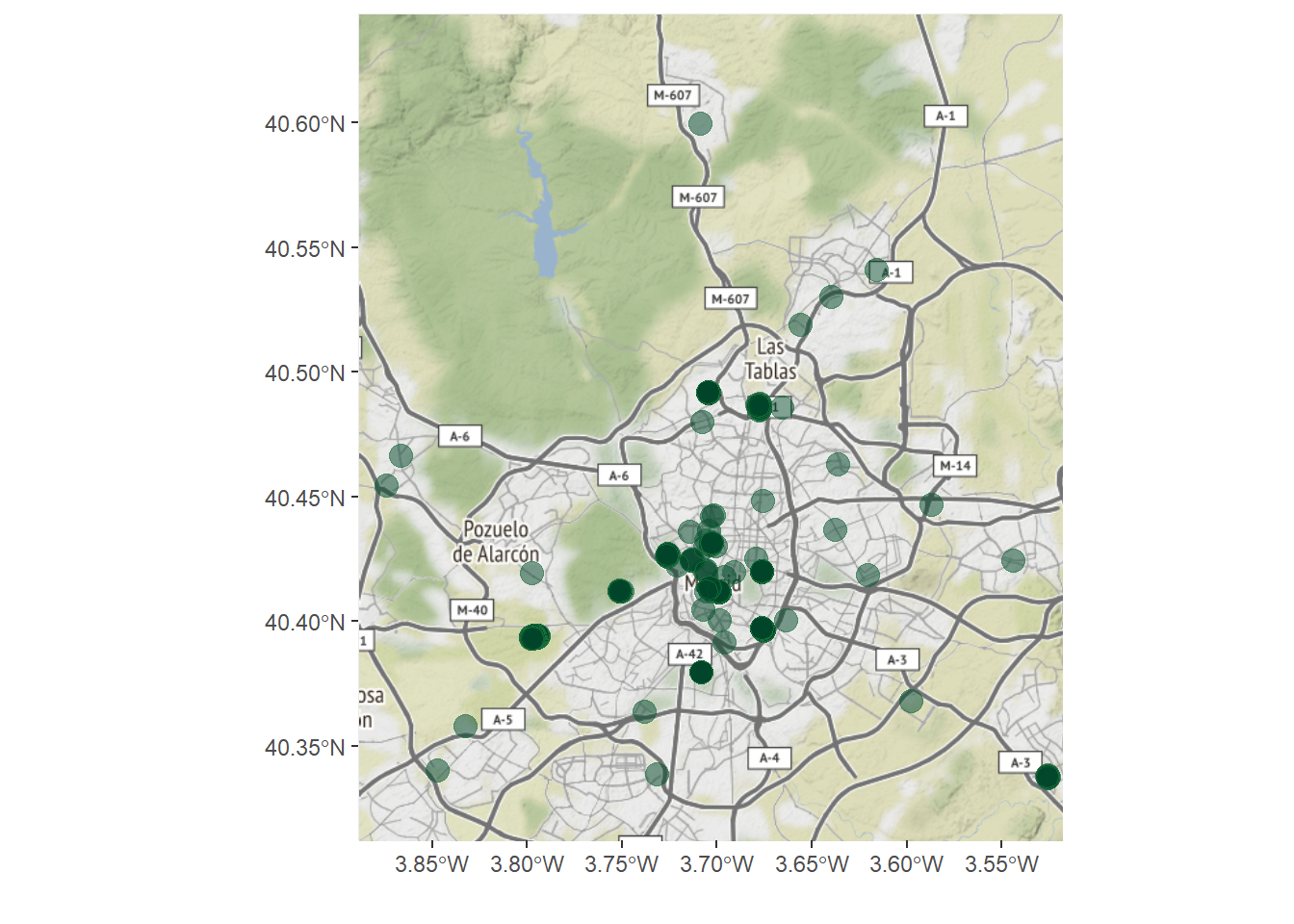
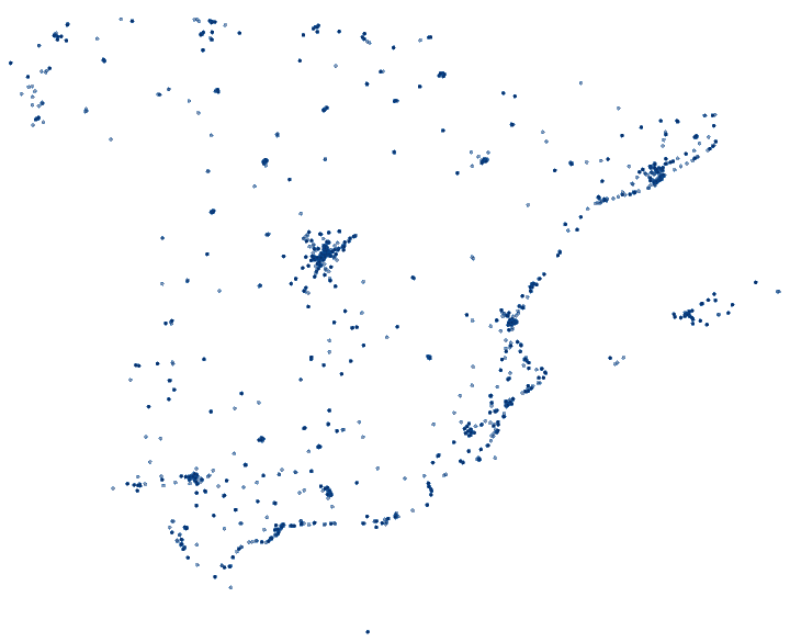
Where can we find Mercadona supermarkets?
Instead of obtaining a bounding box with the function getbb( ) we can build our own box. To do this, we create a vector of four elements, the order has to be West/South/East/North. In the query we use two features: name and shop to filter supermarkets that are of this particular brand. Depending on the area or volume of the query, it is necessary to extend the waiting time. By default, the limit is set at 25 seconds (timeout).
The map, we create in this case, consists only of the supermarket points. Therefore, we use the usual grammar by adding the geometry geom_sf( ). The theme_void( ) function removes everything except for the points.
#bounding box for the Iberian Peninsula
m <- c(-10, 30, 5, 46)

#building the query
q <- m %>%
      opq (timeout = 25*100) %>%
         add_osm_feature("name", "Mercadona") %>%
         add_osm_feature("shop", "supermarket")

#query
mercadona <- osmdata_sf(q)

#final map
ggplot(mercadona$osm_points)+
  geom_sf(colour = "#08519c",
          fill = "#08306b",
          alpha = .5,
          size = 1,
          shape = 21)+
  theme_void()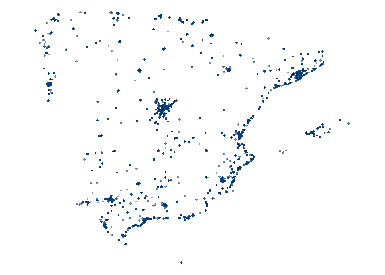
![]()