Firefly cartography
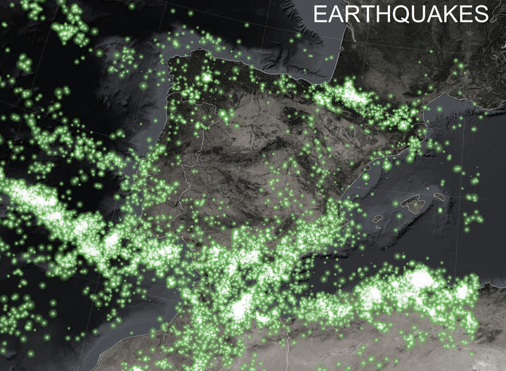
Cartography firefly
Firefly maps are promoted and described by
John Nelson who published a post in 2016 about its characteristics. However, these types of maps are linked to ArcGIS, which has led me to try to recreate them in R. The recent ggplot2 extension ggshadow facilitates the creation of this cartographic style. It is characterized by three elements 1) a dark and unsaturated basemap (eg satellite imagery) 2) a masked vignette and highlighted area and 3) a single bright thematic layer. The essential are the colors and the brightness that is achieved with cold colors, usually neon colors. John Nelson explains more details in this post.
What is the firefly style for? In the words of John Nelson: “the map style that captures our attention and dutifully honors the First Law of Geography”. John refers to what was said by Waldo Tobler “everything is related to everything else, but near things are more related than distant things” (Tobler 1970).
In this post we will visualize all earthquakes recorded in southwestern Europe with a magnitude greater than 3.
Packages
We will use the following packages:
| Package | Description |
|---|---|
| tidyverse | Collection of packages (visualization, manipulation): ggplot2, dplyr, purrr, etc. |
| terra | Import, export and manipulate raster (raster successor package) |
| raster | Import, export and manipulate raster |
| sf | Simple Feature: import, export and manipulate vector data |
| ggshadow | ggplot2 extension for shaded and glow geometries |
| ggspatial | ggplot2 extension for spatial objects |
| ggnewscale | ggplot2 extension to create multiple scales |
| janitor | Simple functions to examine and clean data |
| rnaturalearth | Vector maps of the world ‘Natural Earth’ |
# install the packages if necessary

if(!require("tidyverse")) install.packages("tidyverse")
if(!require("sf")) install.packages("sf")
if(!require("terra")) install.packages("terra")
if(!require("raster")) install.packages("raster")
if(!require("ggshadow")) install.packages("ggshadow")
if(!require("ggspatial")) install.packages("ggspatial")
if(!require("ggnewscale")) install.packages("ggnewscale")
if(!require("janitor")) install.packages("janitor")
if(!require("rnaturalearth")) install.packages("rnaturalearth")

# load packages

library(raster)
library(terra)
library(sf)
library(tidyverse)
library(ggshadow)
library(ggspatial)
library(ggnewscale)
library(janitor)
library(rnaturalearth)
Preparation
Data
First we download all the necessary data. For the base map we will use the Blue Marble imagery via the access to worldview.earthdata.nasa.gov where I have downloaded a selection of the area of interest in geoTiff format with a resolution of 1 km. It is important to adjust the resolution to the necessary detail of the map.
- Blue Marble selection via worldview.earthdata.nasa.gov ( ~ 66 MB) download
- Records of historical earthquakes in southwestern Europe from IGN download
Import
The first thing we do is to import the RGB Blue Marble raster and the earthquake data. To import the raster I use the new package terra which is the successor of the raster package. You can find a recent comparison here. Not all packages are yet compatible with the new SpatRaster class, so we also need the raster package.
# earthquakes

earthquakes <- read.csv2("catalogoComunSV_1621713848556.csv")
str(earthquakes)
## 'data.frame': 149724 obs. of 10 variables:
## $ Evento : chr " 33" " 34" " 35" " 36" ...
## $ Fecha : chr " 02/03/1373" " 03/03/1373" " 08/03/1373" " 19/03/1373" ...
## $ Hora : chr " 00:00:00" " 00:00:00" " 00:00:00" " 00:00:00" ...
## $ Latitud : chr " 42.5000" " 42.5000" " 42.5000" " 42.5000" ...
## $ Longitud : chr " 0.7500" " 0.7500" " 0.7500" " 0.7500" ...
## $ Prof...Km. : int NA NA NA NA NA NA NA NA NA NA ...
## $ Inten. : chr " VIII-IX" " " " " " " ...
## $ Mag. : chr " " " " " " " " ...
## $ Tipo.Mag. : int NA NA NA NA NA NA NA NA NA NA ...
## $ Localización: chr "Ribagorça.L" "Ribagorça.L" "Ribagorça.L" "Ribagorça.L" ...# Blue Marble RGB raster
bm <- rast("snapshot-2017-11-30T00_00_00Z.tiff")
bm # contains three layers (red, green, blue)## class : SpatRaster
## dimensions : 7156, 7156, 3 (nrow, ncol, nlyr)
## resolution : 0.008789272, 0.008789272 (x, y)
## extent : -33.49823, 29.39781, 15.77547, 78.67151 (xmin, xmax, ymin, ymax)
## coord. ref. : lon/lat WGS 84 (EPSG:4326)
## source : snapshot-2017-11-30T00_00_00Z.tiff
## colors RGB : 1, 2, 3
## names : snapshot-2~0_00_00Z_1, snapshot-2~0_00_00Z_2, snapshot-2~0_00_00Z_3# plot
plotRGB(bm)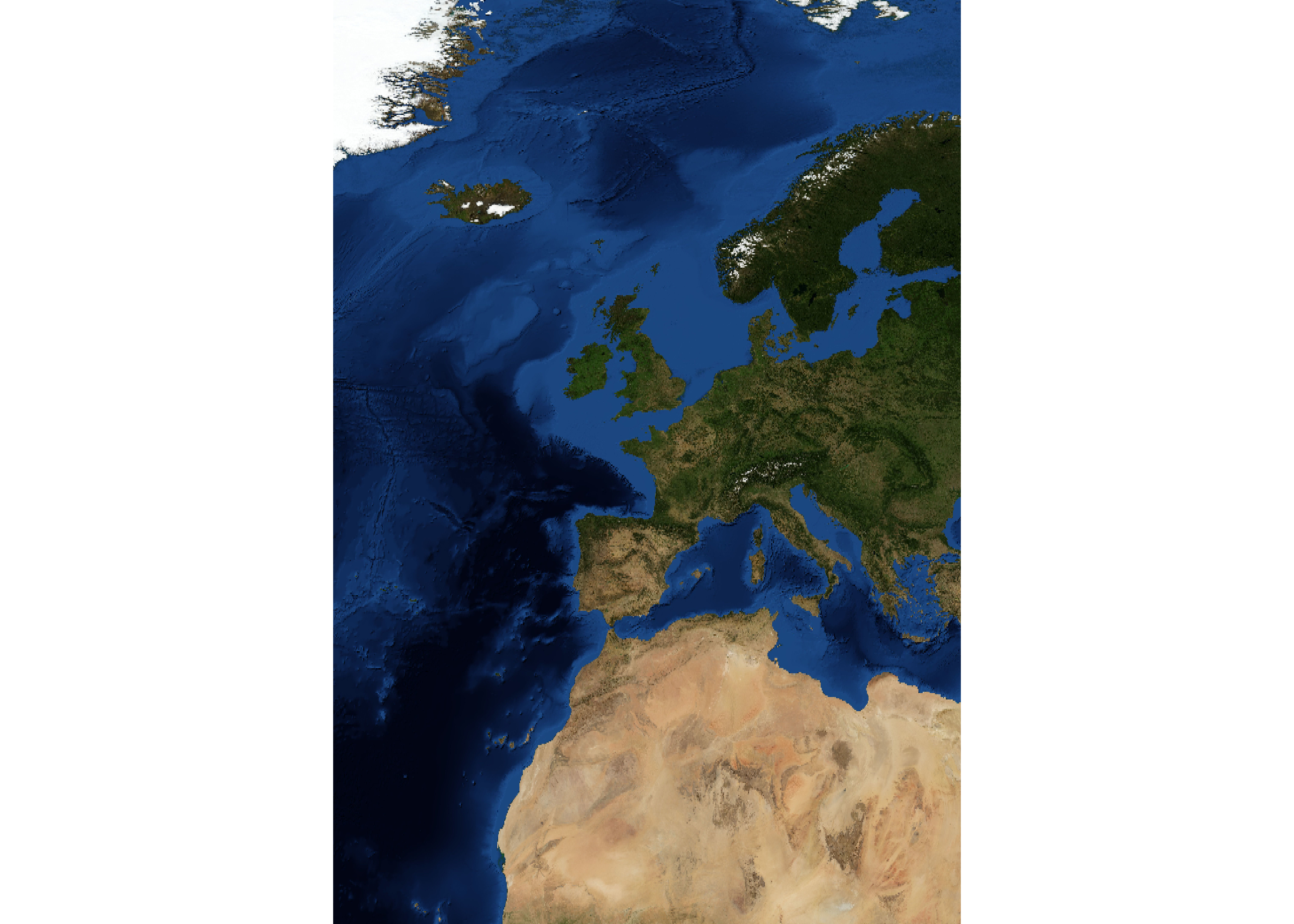
# country boundaries

limits <- ne_countries(scale = 50, returnclass = "sf")
Earthquakes
In this step we clean the imported earthquakes data. 1) We convert longitude, latitude and magnitude into numeric using the parse_number() function and clean the column names with the clean_names() function, 2) We create a spatial object sf and project it using the EPSG:3035 corresponding to ETRS89-extended/LAEA Europe.
# we clean the data and create an sf object

earthquakes <-  earthquakes %>% clean_names() %>%
                  mutate(across(c(mag, latitud, longitud),                                                                                                 parse_number)) %>%
                 st_as_sf(coords = c("longitud", "latitud"),
                       crs = 4326) %>%
                 st_transform(3035) # project to Laea
Blue Marble background Map
We cropped the background map to a smaller extent, but we still haven’t limited to the final area yet.
# clip to the desired area

bm <- crop(bm, extent(-20, 10, 30, 50)) # W, E, S, N
To obtain an unsaturated version of the Blue Marble RGB raster, we must apply a function created for this purpose. In this, we use the colorize(), which helps us converting RGB to HSL and vice versa. The HSL model is defined by Hue, Saturation, Lightness. The last two parameters are expressed in ratio or percentage. The hue is defined on a color wheel from 0 to 360º. 0 is red, 120 is green, 240 is blue. To change the saturation we only have to reduce the value of S.
# apply the function to unsaturate with 5%

bm_desat <- colorize(bm, to = "hsl")
bm_desat[[2]] <- .05 # ratio of saturation
set.RGB(bm_desat, 1:3, "hsl")
bm_desat <- colorize(bm_desat, to = "rgb")

# plot new RGB image

plotRGB(bm_desat)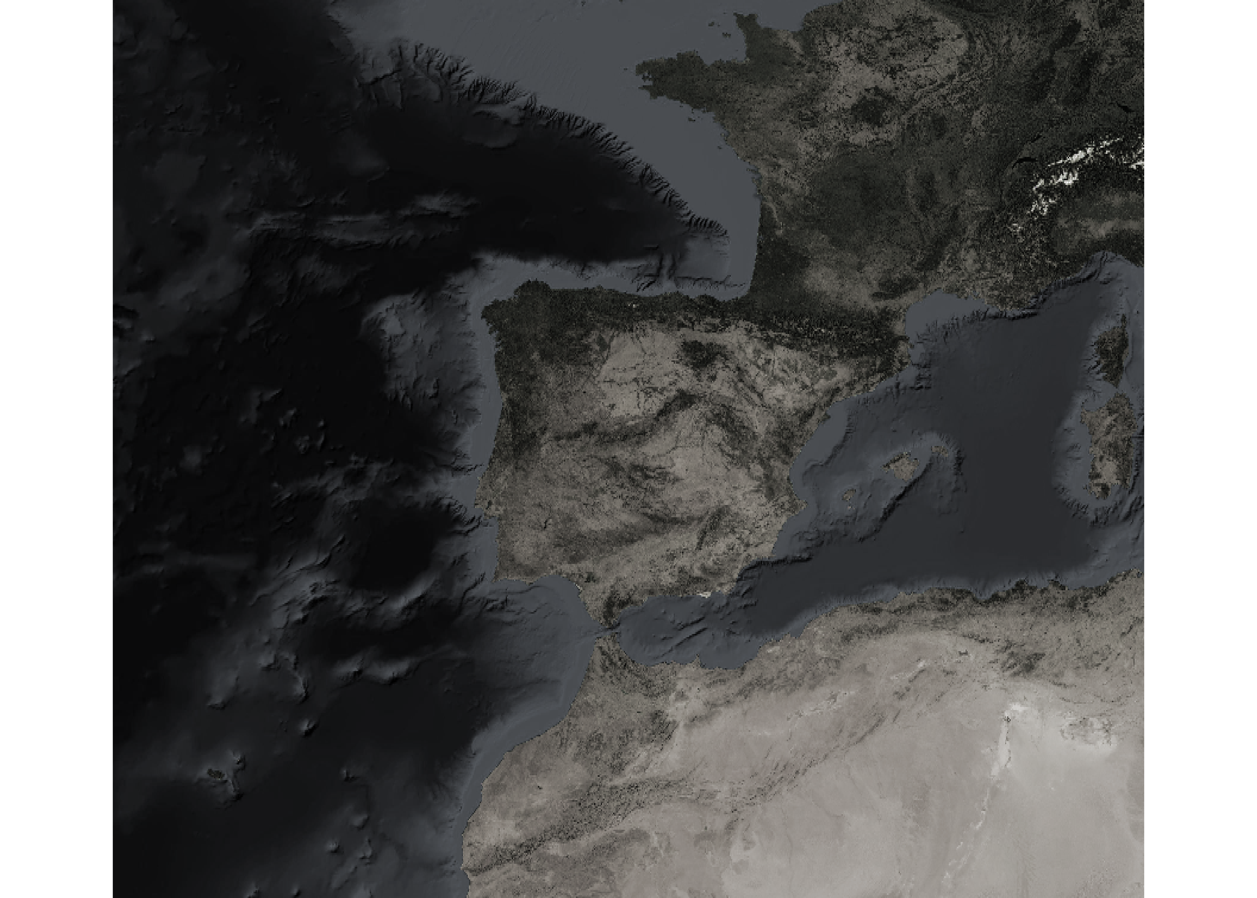
# project

bm_desat <- terra::project(bm_desat, "epsg:3035")
Firefly map construction
Boundaries and graticules
Before starting to build the map, we create graticules and set the final map limits.
# define the final map extent

bx <- tibble(x = c(-13, 6.7), y = c(31, 47)) %>%
       st_as_sf(coords = c("x", "y"), crs = 4326) %>%
        st_transform(3035) %>%
         st_bbox()

# create map graticules

grid <- st_graticule(earthquakes)
Map with image background
The layer_spatial() function of ggspatial allows us to add an RGB raster without major problems, however, it still does not support the newSpatRaster class. Therefore, we must convert it to the stack class with the stack() function. It is also possible to use instead of geom_sf(), the layer_spatial() function for vector objects of class sf orsp.
ggplot() +
  layer_spatial(data = stack(bm_desat)) + # blue marble background map
  geom_sf(data = limits, fill = NA, size = .3, colour = "white") + # country boundaries
  coord_sf(xlim = bx[c(1, 3)],
           ylim = bx[c(2, 4)],
           crs = 3035,
           expand = FALSE) +
  theme_void()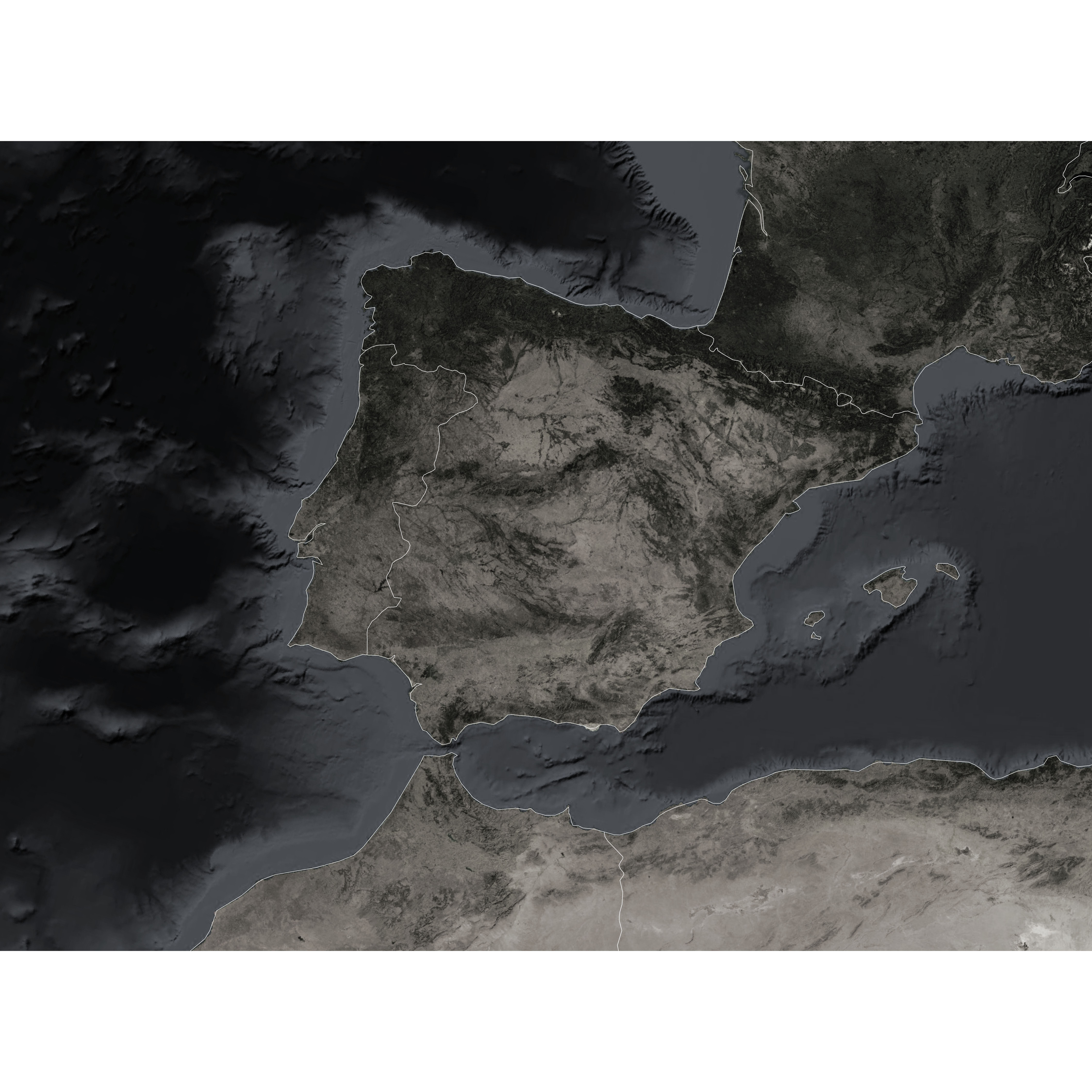
Map with background and earthquakes
To create the glow effect on firefly maps, we use the geom_glowpoint() function from the ggshadow package. There is also the same function for lines. Since our data is of spatial class sf and the geometry sf is not directly supported, we must indicate as an argument stats = "sf_coordinates" and inside aes() indicate geometry = geometry. We will map the size of the points as a function of magnitude. In addition, we filter those earthquakes with a magnitude greater than 3.
Inside the geom_glowpoint() function, 1) we define the desired color for the point and the glow effect, 2) the degree of transparency with alpha either for the point or for the glow. Finally, in the scale_size() function we set the range (minimum, maximum) of the size that the points will have.
ggplot() +
  layer_spatial(data = stack(bm_desat)) +
  geom_sf(data = limits, fill = NA, size = .3, colour = "white") +
  geom_sf(data = grid, colour = "white", size = .1, alpha = .5) +
  geom_glowpoint(data = filter(earthquakes, mag > 3),
                 aes(geometry = geometry, size = mag),
                   alpha = .8,
                   color = "#6bb857",
                   shadowcolour = "#6bb857",
                   shadowalpha = .1,
                   stat = "sf_coordinates",
                   show.legend = FALSE) +
  scale_size(range = c(.1, 1.5)) +
  coord_sf(xlim = bx[c(1, 3)],
           ylim = bx[c(2, 4)],
           crs = 3035,
           expand = FALSE) +
  theme_void()
Final map
The glow effect of firefly maps is characterized by having a white tone or a lighter tone in the center of the points. To achieve this, we must duplicate the previous created layer, changing only the color and make the glow points smaller.
By default, ggplot2 does not allow to use multiple scales for the same characteristic (size, color, etc) of different layers. But the ggnewscale package gives us the ability to incorporate multiple scales of a feature from different layers. The only important thing to achieve this is the order in which each layer (geom) and scale is added. First we must add the geometry and then its corresponding scale. We indicate with new_scale('size') that the next layer and scale is a new one independent of the previous one. If we used color or fill it would be done with new_scale_*().
ggplot() +
  layer_spatial(data = stack(bm_desat)) +
  geom_sf(data = limits, fill = NA, size = .3, colour = "white") +
  geom_sf(data = grid, colour = "white", size = .1, alpha = .5) +
  geom_glowpoint(data = filter(earthquakes, mag > 3),
                   aes(geometry = geometry, size = mag),
                   alpha = .8,
                   color = "#6bb857",
                   shadowcolour = "#6bb857",
                   shadowalpha = .1,
                   stat = "sf_coordinates",
                   show.legend = FALSE) +
  scale_size(range = c(.1, 1.5)) +
  new_scale("size") +
  geom_glowpoint(data = filter(earthquakes, mag > 3),
                   aes(geometry = geometry, size = mag),
                   alpha = .6,
                   shadowalpha = .05,
                   color = "#ffffff",
                   stat = "sf_coordinates",
                   show.legend = FALSE) +
  scale_size(range = c(.01, .7)) +
  labs(title = "EARTHQUAKES") +
  coord_sf(xlim = bx[c(1, 3)], ylim = bx[c(2, 4)], crs = 3035,
           expand = FALSE) +
  theme_void() +
  theme(plot.title = element_text(size = 50, vjust = -5, colour = "white", hjust = .95))
ggsave("firefly_map.png", width = 15, height = 15, units = "in", dpi = 300)